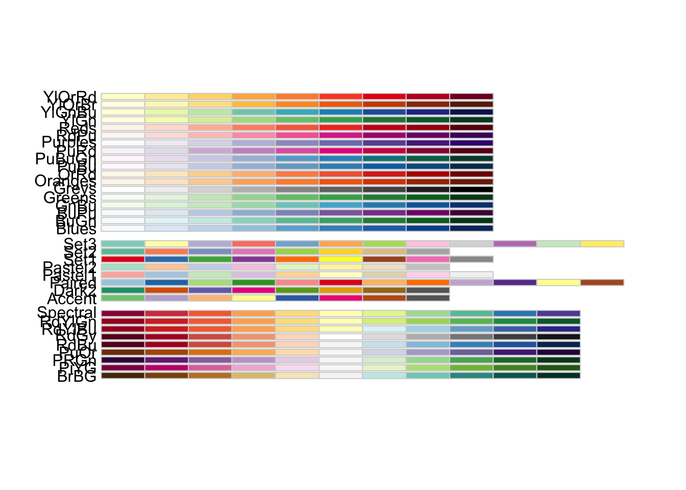
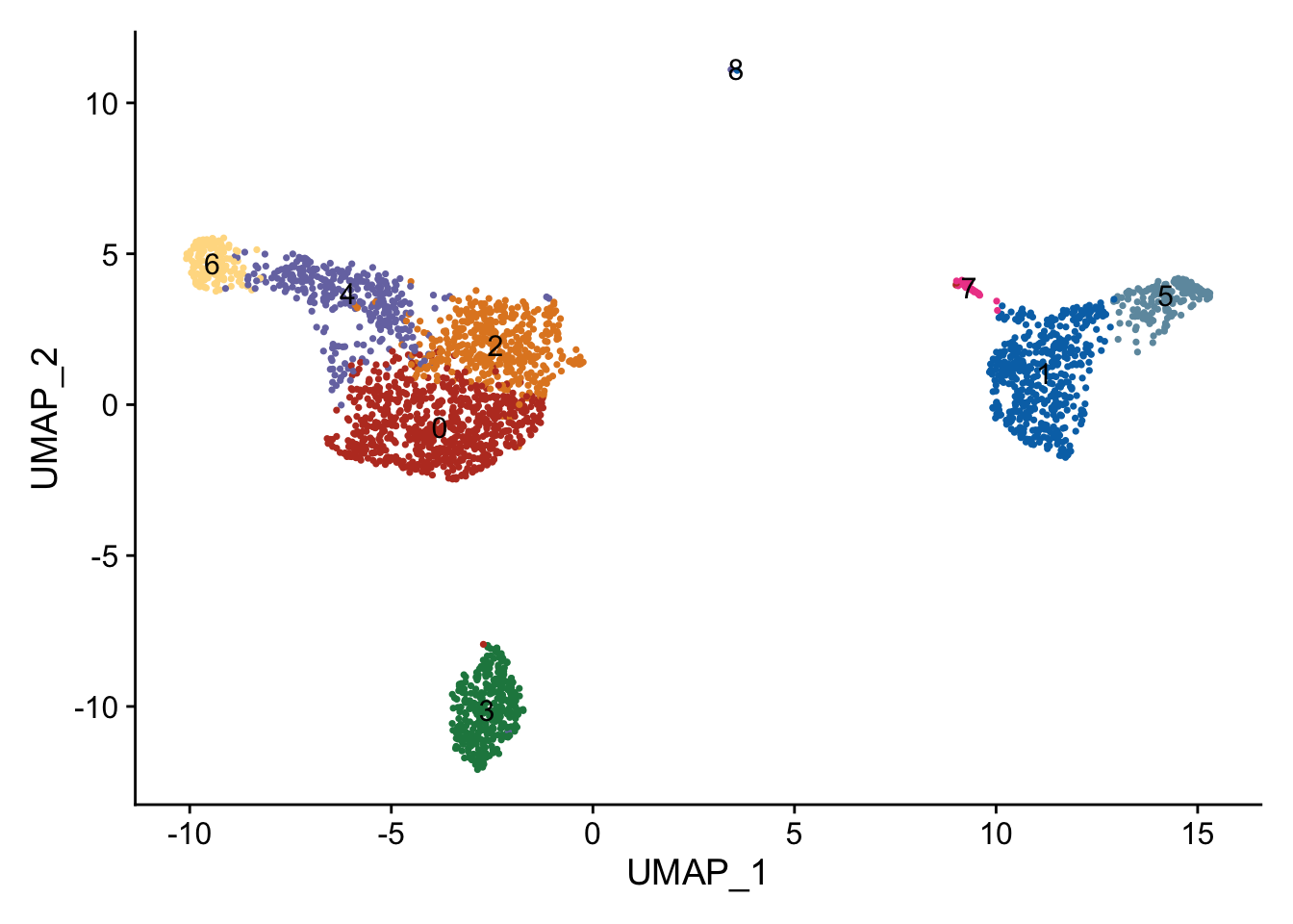
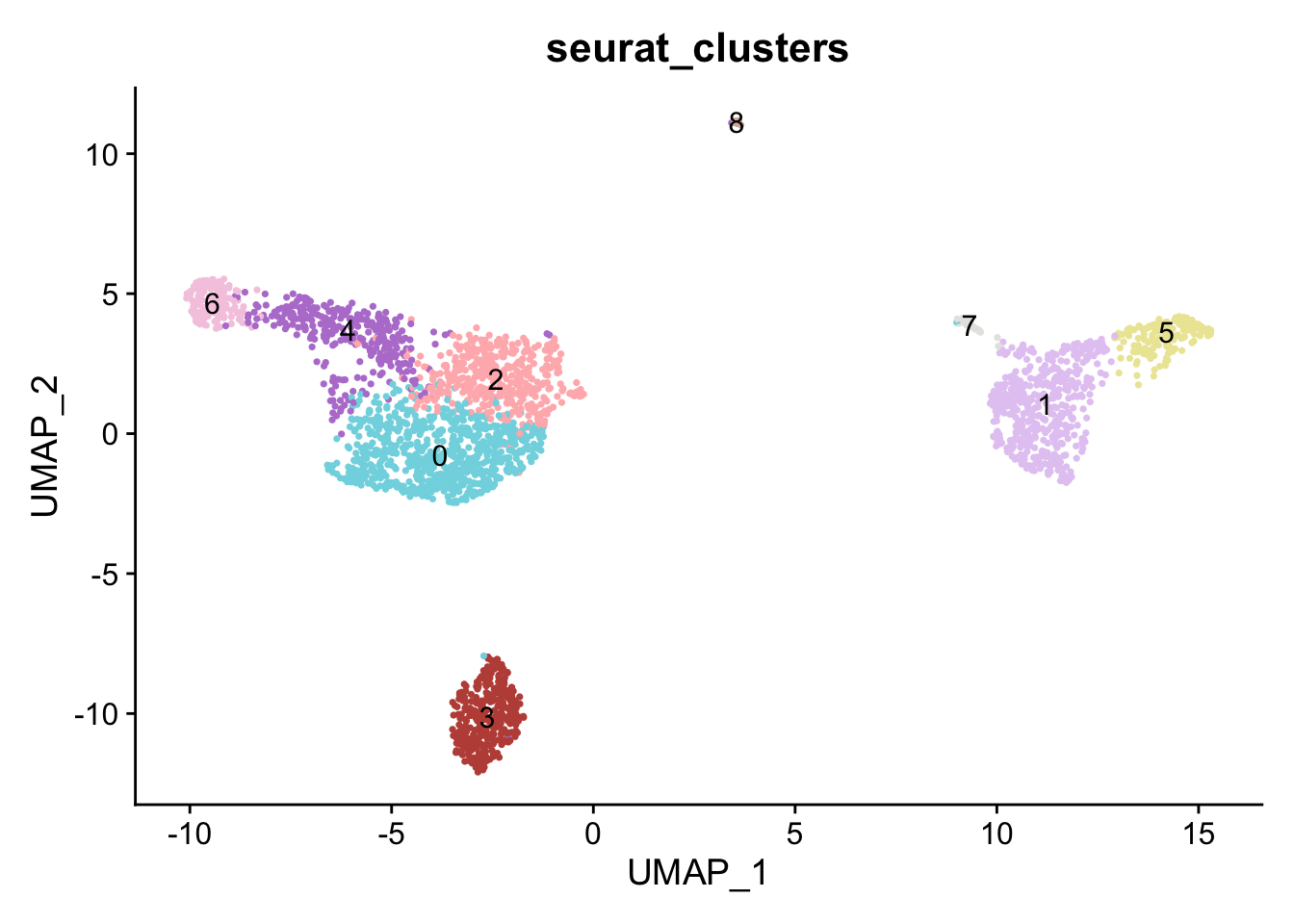
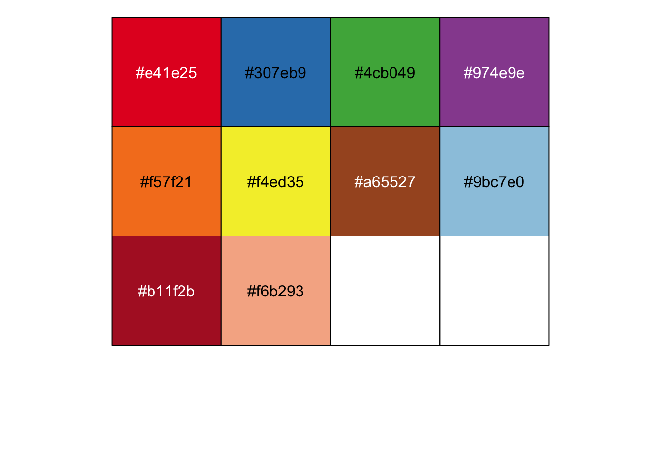
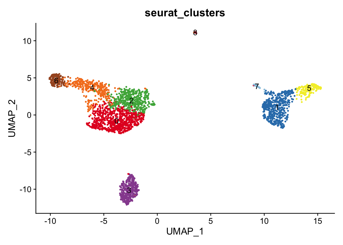
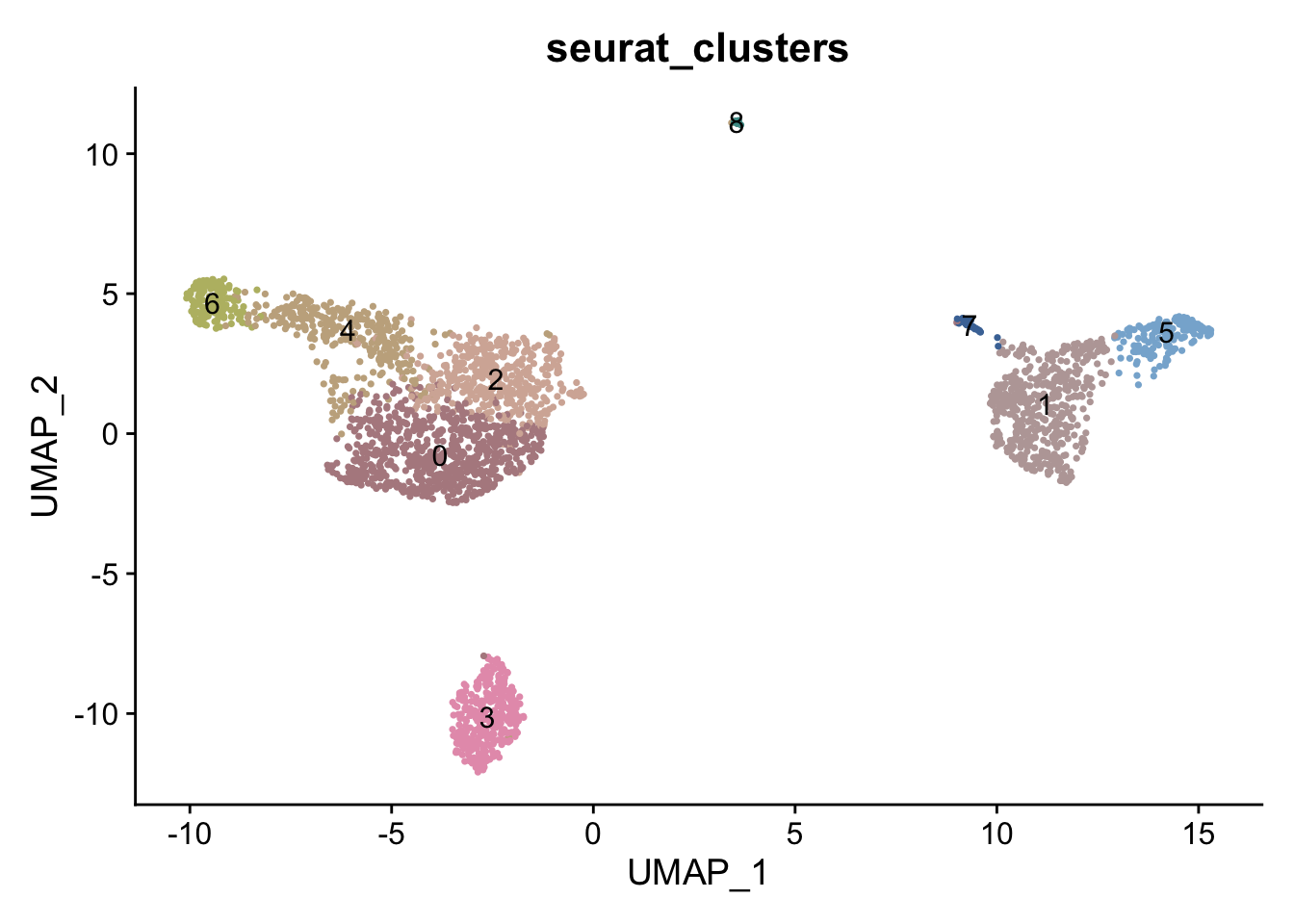
--- title: "Use colorblind-friendly palette for visualization" date: 2023-12-01 date-modified: last-modified categories: - colors - ggplot2 image: colorblind_palette.jpg description: Use ggplot2 to make nice coordinate, colors, and size with friendly colors. --- ```{r setup, include=FALSE} knitr::opts_chunk$set( fig.align = "center", # fig.retina = 3, out.width = "100%", warning = FALSE, # evaluate = FALSE, collapse = TRUE ) ``` ## Color packages 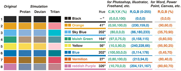 ```{r} #| warning: false #| message: false library (here)library (tidyverse)library (patchwork)library (ggsci)library (Seurat)library (RColorBrewer)library (viridis)library (paletteer)library (cols4all)library (RImagePalette)library (scales)``` ## Basic colors ```{r} # gray colors <- c ("gray" , "lightgray" , "darkgray" , "black" )barplot (1 : 4 , col = cbp)# 4 colors <- c ("#b8b8b8" , "#02ff00" , "#f9a506" , "#ff3c31" barplot (1 : 4 , col = cbp)# 6 colors <- c ("#4C72B0" , "#55A868" , "#C44E52" , "#8172B2" , "#CCB974" , "#64B5CD" barplot (1 : 6 , col = cbp)``` ```{r} # 8 colors <- c ("#999999" , "#E69F00" , "#56B4E9" , "#009E73" , "#F0E442" , "#0072B2" , "#D55E00" , "#CC79A7" barplot (1 : 8 , col = cbp)# 9 colors <- c ("#000000" , "#999999" , "#E69F00" , "#56B4E9" , "#009E73" , "#F0E442" , "#0072B2" , "#D55E00" , "#CC79A7" barplot (1 : 9 , col = cbp)``` ## Color() ```{r} load (here ("projects" , "2023_scRNA_Seurat" , "pbmc_tutorial.RData" ))# 657 colors length (colors ())show_col (colors ()[1 : 50 ])<- c ("#80d7e1" ,"#e4cbf2" ,"#ffb7ba" ,"#bf5046" ,"#b781d2" ,"#ece7a3" , "#f5cbe1" ,"#e6e5e3" ,"#d2b5ab" ,"#d9e3f5" ,"#f29432" ,"#9c9895" show_col (cbp)## Single cell plot <- DimPlot (pbmc, reduction = "umap" ,label = T) + NoLegend ()<- DimPlot (pbmc, reduction = "umap" ,cols = cbp,label = T)+ NoLegend ()+ p2``` ## RColorBrewer ```{r} library (RColorBrewer)display.brewer.all ()<- brewer.pal (9 , "Set1" )<- brewer.pal (9 , "Set1" )<- brewer.pal (8 , "Set2" )<- c (b1,b2) ``` ## ggsci ```{r} library (ggsci)# vignette("ggsci") DimPlot (pbmc, reduction = "umap" , label = TRUE ) + scale_color_nejm () + NoLegend ()<- pal_nejm ("default" , alpha = 0.5 )(8 ) ``` ## paletteer ```{r} library (paletteer) paletteer_c ("scico::berlin" , n = 10 )paletteer_d ("RColorBrewer::Paired" ,n= 12 )paletteer_dynamic ("cartography::green.pal" , 20 )``` ## cols4all ```{r} # remotes::install_github("mtennekes/cols4all") library (cols4all)# c4a_gui() <- c4a ("light24" , 9 )``` ```{r} # Color from:Nat Med. 2019 Aug;25(8):1251-1259. <- c ("#80d7e1" ,"#e4cbf2" ,"#ffb7ba" ,"#bf5046" ,"#b781d2" ,"#ece7a3" ,"#f5cbe1" ,"#e6e5e3" ,"#d2b5ab" ,"#d9e3f5" ,"#f29432" ,"#9c9895" show_col (cbp, labels = TRUE )DimPlot (pbmc, reduction = "umap" , group.by= 'seurat_clusters' , label = T) + scale_color_manual (values = cbp)+ NoLegend ()# Color from:Immunity. 2020 May 19;52(5):808-824.e7. <- c ("#e41e25" ,"#307eb9" ,"#4cb049" ,"#974e9e" ,"#f57f21" ,"#f4ed35" ,"#a65527" ,"#9bc7e0" ,"#b11f2b" ,"#f6b293" show_col (cbp, labels = TRUE )DimPlot (pbmc, reduction = "umap" , group.by= 'seurat_clusters' , label= T) + scale_color_manual (values = cbp)+ NoLegend ()# Color from:Cell. 2019 Oct 31;179(4):829-845.e20. <- c ("#b38a8f" ,"#bba6a6" ,"#d5b3a5" ,"#e69db8" ,"#c5ae8d" ,"#87b2d4" ,"#babb72" ,"#4975a5" ,"#499994" ,"#8e8786" ,"#93a95d" ,"#f19538" ,"#fcba75" ,"#8ec872" ,"#ad9f35" ,"#8ec872" ,"#d07794" ,"#ff9796" ,"#b178a3" ,"#e56464" ,"#6cb25e" ,"#ca9abe" ,"#d6b54c" show_col (cbp, labels = TRUE )DimPlot (pbmc, reduction = "umap" , group.by= 'seurat_clusters' , label = T) + scale_color_manual (values = cbp) + NoLegend ()``` ## Pick color from images ```{r} #| eval: false # devtools::install_github("joelcarlson/RImagePalette") library (RImagePalette)<- jpeg:: readJPEG ("color.jpg" )display_image (lifeAquatic)<- image_palette (lifeAquatic, n= 16 ) show_col (mycolor)```