in Python, understanding data types and structures is essential for writting effective code. Data types determine the kind of data a variable can hold, while data structures allow you to organize and manage that data efficiently.
Numbers: Represent numerical values, including integers and floating-point numbers.
Strings: Represent sequences of characters, used for text manipulation.
Booleans: Represent truth values, either True or False.
Lists: Ordered collections of items, allowing for duplicate values and mutable operations.
Tuples: Ordered collections of items, similar to lists but immutable.
Sets: Unordered collections of unique items, useful for membership testing and eliminating duplicates.
Dictionaries: Unordered, Key-value pairs that allow for efficient data retrieval based on unique keys.
## Numbers and stringsinteger_num =42float_num =3.14string_text ="Hello, Python!"## List: mutable, ordered collectionfruits = ["apple", "banana", "cherry"]## Tuple: immutable, ordered collectiondimensions = (1920, 1080)## Dictionary: unordered, key-value pairsperson = {"name": "Alice", "age": 30, "city": "New York"}## Set: unordered collection of unique itemsunique_numbers = {1, 2, 3, 4, 5}print("Integer:", integer_num)print("Float:", float_num)print("String:", string_text)print("List of fruits:", fruits)print("Tuple of dimensions:", dimensions)print("Dictionary of person:", person)print("Set of unique numbers:", unique_numbers)
Integer: 42
Float: 3.14
String: Hello, Python!
List of fruits: ['apple', 'banana', 'cherry']
Tuple of dimensions: (1920, 1080)
Dictionary of person: {'name': 'Alice', 'age': 30, 'city': 'New York'}
Set of unique numbers: {1, 2, 3, 4, 5}
in R, the list is a versatile container type that can hold elements of different types and structures.
There is no single direct equivalent of R’s list in Python that support all the same features.
Instead, there are (at least) 4 different Python container types we need to aware:
list: ordered, mutable, allows duplicate elements, created using []
tuple: ordered, immutable, allows duplicate elements, created using ()
set: unordered, mutable, no duplicate elements, created using {}
dict: unordered, mutable, key-value pairs, created using {}
Lists
Python lists created using bare brackets [], closer to R’s as.list function.
The most important thing to know about Python lists is that they are mutable.
x = [1, 2, 3]y = x # `y` and `x` now refer to the same list!x.append(4)print("x is", x)#> x is [1, 2, 3, 4]print("y is", y)#> y is [1, 2, 3, 4]
Some syntactic sugar around Python lists you might encounter is the usage of + and * with lists. These are concatenation and replication operators, akin to R’s c() and rep().
x = [1]x#> [1]x + x#> [1, 1]x *3#> [1, 1, 1]
Index into lists with integers using trailing [], but note that indexing is 0-based
x = [1, 2, 3]x[0]#> 1x[1]#> 2x[2]#> 3try: x[3]exceptExceptionas e:print(e)#> list index out of range## Negative numbers count from the end of the listx[-1]#> 3x[-2]#> 2x[-3]#> 1
Slice ranges of lists using : inside the trailing []. Note that the end index is exclusive. We can optionally specify a stride using a second :.
x = [1, 2, 3, 4, 5, 6]x[0:2] # get items at index positions 0, 1#> [1, 2]x[1:] # get items from index position 1 to the end#> [2, 3, 4, 5, 6]x[:-2] # get items from beginning up to the 2nd to last.#> [1, 2, 3, 4]x[:] # get all the items (idiom used to copy the list so as not to modify in place)#> [1, 2, 3, 4, 5, 6]x[::2] # get all the items, with a stride of 2#> [1, 3, 5]x[1::2] # get all the items from index 1 to the end, with a stride of 2#> [2, 4, 6]
Tuples
Tuples behave like lists, but are immutable (cannot be changed after creation).
Created using bare parentheses (), but parentheses are not strictly required.
x = (1, 2) # tuple of length 2type(x)#> <class 'tuple'>len(x)#> 2x#> (1, 2)x = (1,) # tuple of length 1type(x)#> <class 'tuple'>len(x)#> 1x#> (1,)x = () # tuple of length 0print(f"{type(x) =}; {len(x) =}; {x =}")#> type(x) = <class 'tuple'>; len(x) = 0; x = ()# example of an interpolated string literalsx =1, 2# also a tupletype(x)#> <class 'tuple'>len(x)#> 2x =1, # beware a single trailing comma! This is a tuple!type(x)#> <class 'tuple'>len(x)#> 1
Tuples are the container that powers the packing and unpacking semantics in Python.
Packing and unpacking tuples is a common idiom in Python.
Python provides the convenience of unpacking tuples into multiple variables in a single statement.
x = (1, 2, 3)a, b, c = xa#> 1b#> 2c#> 3
Tuple unpacking can occur in a variety of contexts, such as iteration:
Python raises an error when attampt to unpack a container to the wrong number of symbols:
x = (1, 2, 3)a, b, c, =x # successa, b = x # error, x has too many values to unpack#> ValueError: too many values to unpack (expected 2)a, b, c, d = x # error, x has not enough values to unpack#> ValueError: not enough values to unpack (expected 4, got 3)
Unpack a variable number of values using the * operator:
Sets are a container that can be used to efficiently track unique items or deduplicate lists. They are constructed using {val1, val2} (like a dictionary, but without :). Think of them as dictionary where you only use the keys. Sets have many efficient methods for membership operations, like intersection(), issubset(), union() and so on.
Control flow in Python allows you to make decisions and execute different blocks of code based on conditions. Loops enable you to repeat a block of code multiple times.
Best practices for control flow and loops include: - Keep conditions simple and clear. Break down complex conditions into smaller parts. - Use meaningful variable names to enhance readability. - Avoid deeply nested loops and conditions to maintain code clarity. - Use comments to explain the purpose of complex conditions or loops. - Test edge cases to ensure your control flow behaves as expected.
# Conditional statementsx =10if x >5:print("x is greater than 5")elif x ==5:print("x is equal to 5")else:print("x is less than 5")
Iteration
## For loop: iterating over a listfor i inrange(5):print("Iteration:", i)## While loop: continues until a condition is metcount =0while count <5:print("Count is:", count) count +=1
Conditional execution in Python is achieved using the if/else construct (if and else are reserved words).
# Conidtional executionx =10if x >10:print("I am a big number")else:print("I am a small number")# Multi-way if/elsex =10if x >10:print("I am a big number")elif x >5:print("I am kind of small")else:print("I am really number")
Loops
Two looping constructs in Python
For : used when the number of possible iterations (repetitions) are known in advance
While: used when the number of possible iterations (repetitions) can not be defined in advance. Can lead to infinite loops, if conditions are not handled properly
for customer in ["John", "Mary", "Jane"]:print("Hello ", customer)print("Please pay") collectCash() giveGoods()hour_of_day =9while hour_of_day <17: moveToWarehouse() locateGoods() moveGoodsToShip() hour_of_day = getCurrentTime()
What happens if you need to stop early? We use the break keyword to do this.
It stops the iteration immediately and moves on to the statement that follows the looping
What happens when you want to just skip the rest of the steps? We can use the continue keyword for this.
It skips the rest of the steps but moves on to the next iteration.
for customer in ["John", "Mary", "Jane"]:print("Hello ", customer)print("Please pay") paid = collectCash()if paid ==False:continue giveGoods()
Exceptions
Exceptions are errors that are found during execution of the Python program.
They typically cause the program to fail.
However we can handle them using the ‘try/except’ construct.
num =input("Please enter a number: ")try: num =int(num)print("number squared is "+str(num**2))except:print("You did not enter a valid number")
help()type()len()range()list()tuple()dict()
Dataframe
#| eval: true## Python's dataframe comes form the pandas libraryimport pandas as pd## It's actually a type of dictionary of listspy_df = pd.DataFrame( {'Name': ['Alice', 'Bob', 'Charlie'],'Age': [25, 30, 35],'City': ['New York', 'Los Angeles', 'Chicago'] })print(py_df)
---title: Python Programmingdate: 2020-09-09published-title: Createddate-modified: last-modifiedtitle-block-banner: "#212529"toc-title: "Contents"---## Data Stuctures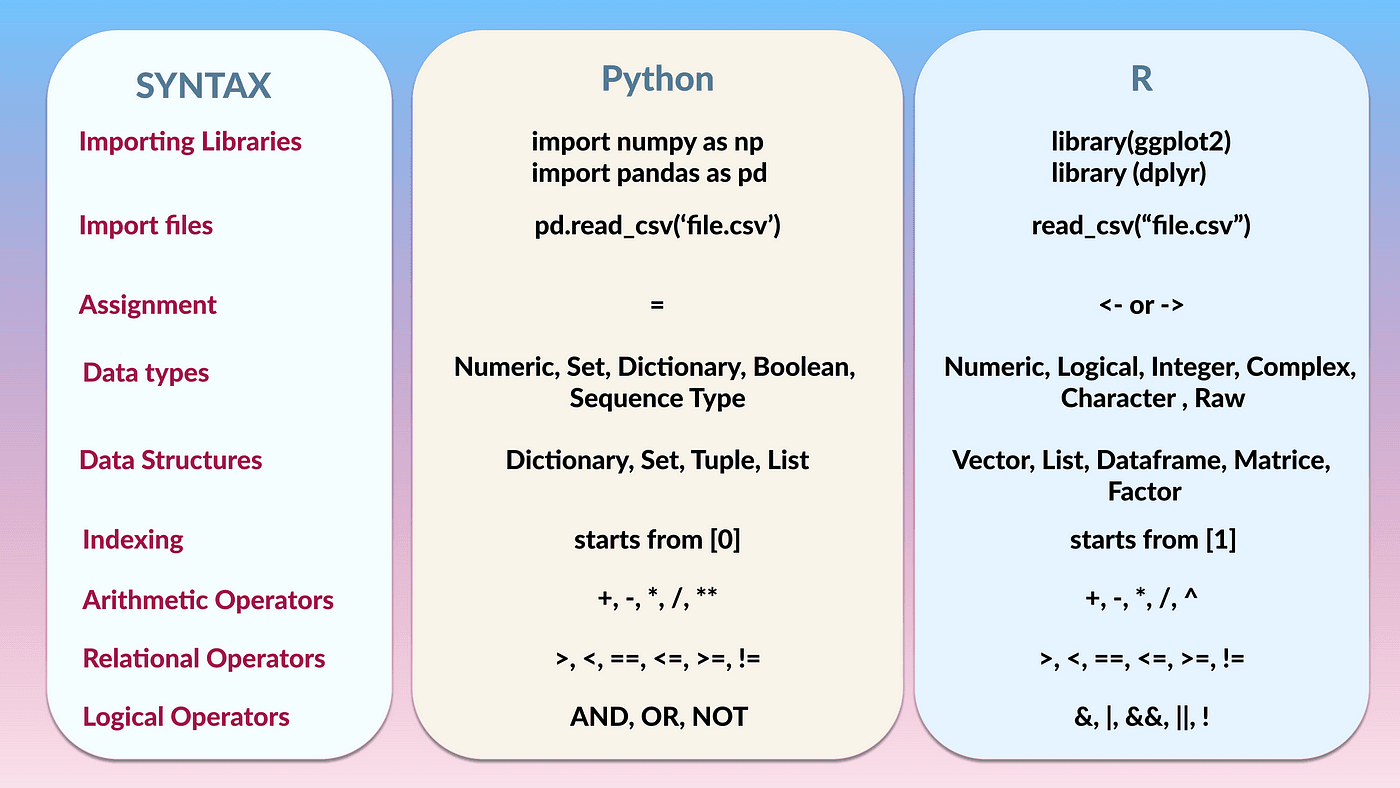{width=800px}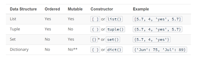{width=800px}in Python, understanding data types and structures is essential for writtingeffective code. Data types determine the kind of data a variable can hold,while data structures allow you to organize and manage that data efficiently.- Numbers: Represent numerical values, including integers and floating-point numbers.- Strings: Represent sequences of characters, used for text manipulation.- Booleans: Represent truth values, either True or False.- Lists: Ordered collections of items, allowing for duplicate values and mutable operations.- Tuples: Ordered collections of items, similar to lists but immutable.- Sets: Unordered collections of unique items, useful for membership testing and eliminating duplicates.- Dictionaries: Unordered, Key-value pairs that allow for efficient data retrieval based on unique keys.```{python}## Numbers and stringsinteger_num =42float_num =3.14string_text ="Hello, Python!"## List: mutable, ordered collectionfruits = ["apple", "banana", "cherry"]## Tuple: immutable, ordered collectiondimensions = (1920, 1080)## Dictionary: unordered, key-value pairsperson = {"name": "Alice", "age": 30, "city": "New York"}## Set: unordered collection of unique itemsunique_numbers = {1, 2, 3, 4, 5}print("Integer:", integer_num)print("Float:", float_num)print("String:", string_text)print("List of fruits:", fruits)print("Tuple of dimensions:", dimensions)print("Dictionary of person:", person)print("Set of unique numbers:", unique_numbers)```* in R, the `list` is a versatile container type that can hold elements of different types and structures.* There is no single direct equivalent of R's `list` in Python that support all the same features.* Instead, there are (at least) 4 different Python container types we need to aware: + `list`: ordered, mutable, allows duplicate elements, created using `[]` + `tuple`: ordered, immutable, allows duplicate elements, created using `()` + `set`: unordered, mutable, no duplicate elements, created using `{}` + `dict`: unordered, mutable, key-value pairs, created using `{}`### ListsPython lists created using bare brackets `[]`, closer to R's `as.list` function.* The most important thing to know about Python lists is that they are mutable.```{python}#| eval: falsex = [1, 2, 3]y = x # `y` and `x` now refer to the same list!x.append(4)print("x is", x)#> x is [1, 2, 3, 4]print("y is", y)#> y is [1, 2, 3, 4]```* Some syntactic sugar around Python lists you might encounter is the usage of + and * with lists.These are concatenation and replication operators, akin to R’s c() and rep().```{python}#| eval: falsex = [1]x#> [1]x + x#> [1, 1]x *3#> [1, 1, 1]```* Index into lists with integers using trailing `[]`, but note that indexing is 0-based```{python}#| eval: falsex = [1, 2, 3]x[0]#> 1x[1]#> 2x[2]#> 3try: x[3]exceptExceptionas e:print(e)#> list index out of range## Negative numbers count from the end of the listx[-1]#> 3x[-2]#> 2x[-3]#> 1```* Slice ranges of lists using `:` inside the trailing `[]`. Note that the end index is exclusive. We can optionally specify a stride using a second `:`.```{python}#| eval: falsex = [1, 2, 3, 4, 5, 6]x[0:2] # get items at index positions 0, 1#> [1, 2]x[1:] # get items from index position 1 to the end#> [2, 3, 4, 5, 6]x[:-2] # get items from beginning up to the 2nd to last.#> [1, 2, 3, 4]x[:] # get all the items (idiom used to copy the list so as not to modify in place)#> [1, 2, 3, 4, 5, 6]x[::2] # get all the items, with a stride of 2#> [1, 3, 5]x[1::2] # get all the items from index 1 to the end, with a stride of 2#> [2, 4, 6]```### Tuples* Tuples behave like lists, but are immutable (cannot be changed after creation).* Created using bare parentheses `()`, but parentheses are not strictly required.```{python}#| eval: false#| output: asisx = (1, 2) # tuple of length 2type(x)#> <class 'tuple'>len(x)#> 2x#> (1, 2)x = (1,) # tuple of length 1type(x)#> <class 'tuple'>len(x)#> 1x#> (1,)x = () # tuple of length 0print(f"{type(x) =}; {len(x) =}; {x =}")#> type(x) = <class 'tuple'>; len(x) = 0; x = ()# example of an interpolated string literalsx =1, 2# also a tupletype(x)#> <class 'tuple'>len(x)#> 2x =1, # beware a single trailing comma! This is a tuple!type(x)#> <class 'tuple'>len(x)#> 1```* Tuples are the container that powers the packing and unpacking semantics in Python. + Packing and unpacking tuples is a common idiom in Python. + Python provides the convenience of unpacking tuples into multiple variables in a single statement.```{python}#| eval: falsex = (1, 2, 3)a, b, c = xa#> 1b#> 2c#> 3```Tuple unpacking can occur in a variety of contexts, such as iteration:```{python}#| eval: falsexx = (("a", 1), ("b", 2))for x1, x2 in xx:print("x1 = ", x1)print("x2 = ", x2)#> x1 = a#> x2 = 1#> x1 = b#> x2 = 2```Python raises an error when attampt to unpack a container to the wrong number of symbols:```{python}#| eval: falsex = (1, 2, 3)a, b, c, =x # successa, b = x # error, x has too many values to unpack#> ValueError: too many values to unpack (expected 2)a, b, c, d = x # error, x has not enough values to unpack#> ValueError: not enough values to unpack (expected 4, got 3)```Unpack a variable number of values using the `*` operator:```{python}#| eval: falsex = (1, 2, 3)a, *the_rest = xa#> 1the_rest#> [2, 3]```Unpack the nested structures:```{python}#| eval: falsex = ((1, 2), (3, 4))(a, b), (c, d) = x```### SetsSets are a container that can be used to efficiently track unique items or deduplicate lists. They are constructed using `{val1, val2}` (like a dictionary, but without `:`). Think of them as dictionary where you only use the keys. Sets have many efficient methods for membership operations, like `intersection()`, `issubset()`, `union()` and so on.```{python}#| eval: falses = {1, 2, 3}type(s)#> <class 'set'>s#> {1, 2, 3}s.add(1)s#> {1, 2, 3}```### Dictionaries* Dictionaries can be created using syntax like {key: value, key: value, ...}.* Note that `r_to_py` converts R named lists to Python dictionaries.```{python}#| eval: falsed = {"key1": 1,"key2": 2 }d2 = dd#> {'key1': 1, 'key2': 2}d["key1"]#> 1d["key3"] =3d2 # modified in place!#> {'key1': 1, 'key2': 2, 'key3': 3}```* Cannot index into dictionaries using integer indices. Instead, use the keys.```{python}#| eval: falsed = {"key1": 1, "key2": 2}d[1] # error# > KeyError: 1```## Control flowControl flow in Python allows you to make decisions and execute different blocks of code based on conditions.Loops enable you to repeat a block of code multiple times.Best practices for control flow and loops include:- Keep conditions simple and clear. Break down complex conditions into smaller parts.- Use meaningful variable names to enhance readability.- Avoid deeply nested loops and conditions to maintain code clarity.- Use comments to explain the purpose of complex conditions or loops.- Test edge cases to ensure your control flow behaves as expected.```{python}#| eval: false# Conditional statementsx =10if x >5:print("x is greater than 5")elif x ==5:print("x is equal to 5")else:print("x is less than 5")```## Iteration```{python}#| eval: false## For loop: iterating over a listfor i inrange(5):print("Iteration:", i)## While loop: continues until a condition is metcount =0while count <5:print("Count is:", count) count +=1```Conditional execution in Python is achieved using the if/else construct (if and else are reserved words).```{python}#| eval: false# Conidtional executionx =10if x >10:print("I am a big number")else:print("I am a small number")# Multi-way if/elsex =10if x >10:print("I am a big number")elif x >5:print("I am kind of small")else:print("I am really number")```## LoopsTwo looping constructs in Python- `For` : used when the number of possible iterations (repetitions) are known in advance- `While`: used when the number of possible iterations (repetitions) can not be defined in advance. Can lead to infinite loops, if conditions are not handled properly```{python}#| eval: falsefor customer in ["John", "Mary", "Jane"]:print("Hello ", customer)print("Please pay") collectCash() giveGoods()hour_of_day =9while hour_of_day <17: moveToWarehouse() locateGoods() moveGoodsToShip() hour_of_day = getCurrentTime()```What happens if you need to stop early? We use the `break` keyword to do this.It stops the iteration immediately and moves on to the statement that follows the looping```{python}#| eval: falsewhile hour_of_day <17:if shipIsFull() ==True:break moveToWarehouse() locateGoods() moveGoodsToShip() hour_of_day = getCurrentTime()collectPay()```What happens when you want to just skip the rest of the steps? We can use the `continue` keyword for this.It skips the rest of the steps but moves on to the next iteration.```{python}#| eval: falsefor customer in ["John", "Mary", "Jane"]:print("Hello ", customer)print("Please pay") paid = collectCash()if paid ==False:continue giveGoods()```## Exceptions- Exceptions are errors that are found during execution of the Python program.- They typically cause the program to fail.- However we can handle them using the ‘try/except’ construct.```{python}#| eval: falsenum =input("Please enter a number: ")try: num =int(num)print("number squared is "+str(num**2))except:print("You did not enter a valid number")``````{python}#| eval: falsehelp()type()len()range()list()tuple()dict()```## Dataframe```{.python}#| eval: true## Python's dataframe comes form the pandas libraryimport pandas as pd## It's actually a type of dictionary of listspy_df = pd.DataFrame( { 'Name': ['Alice', 'Bob', 'Charlie'], 'Age': [25, 30, 35], 'City': ['New York', 'Los Angeles', 'Chicago'] })print(py_df)```

