
### load packages
library(rhdf5) # provides functions for handling hdf5 file formats (kallisto outputs bootstraps in this format)
library(tidyverse) # Hadley Wickham's collection of R packages for data science, which we will use throughout the course
library(tximport) # package for getting Kallisto results into R
library(ensembldb) # helps deal with ensembl
library(EnsDb.Hsapiens.v86) # replace with your organism-specific database package
library(here) # file path
library(datapasta) # paste data into R from clipboard
library(edgeR) # well known package for differential expression analysis, but we only use for the DGEList object and for normalization methods
library(matrixStats) # easily calculate stats on rows or columns of a data matrix
library(cowplot) # allows you to combine multiple plots in one figure
library(DT) # for making interactive tables
library(plotly) # for making interactive plots
library(gt) # A layered 'grammar of tables' - think ggplot, but for tables
library(limma) # venerable package for differential gene expression using linear modeling
library(edgeR)
library(RColorBrewer) # need colors to make heatmaps
# library(gameofthrones) #because...why not. Install using 'devtools::install_github("aljrico/gameofthrones")'
library(heatmaply) #for making interactive heatmaps using plotly
library(gplots)
# library(d3heatmap) # for making interactive heatmaps using D3
library(GSEABase) # functions and methods for Gene Set Enrichment Analysis
library(Biobase) # base functions for bioconductor; required by GSEABase
library(GSVA) # Gene Set Variation Analysis, a non-parametric and unsupervised method for estimating variation of gene set enrichment across samples.
library(gprofiler2) # tools for accessing the GO enrichment results using g:Profiler web resources
library(clusterProfiler) # provides a suite of tools for functional enrichment analysis
library(msigdbr) # access to msigdb collections directly within R
library(enrichplot) # great for making the standard GSEA enrichment plots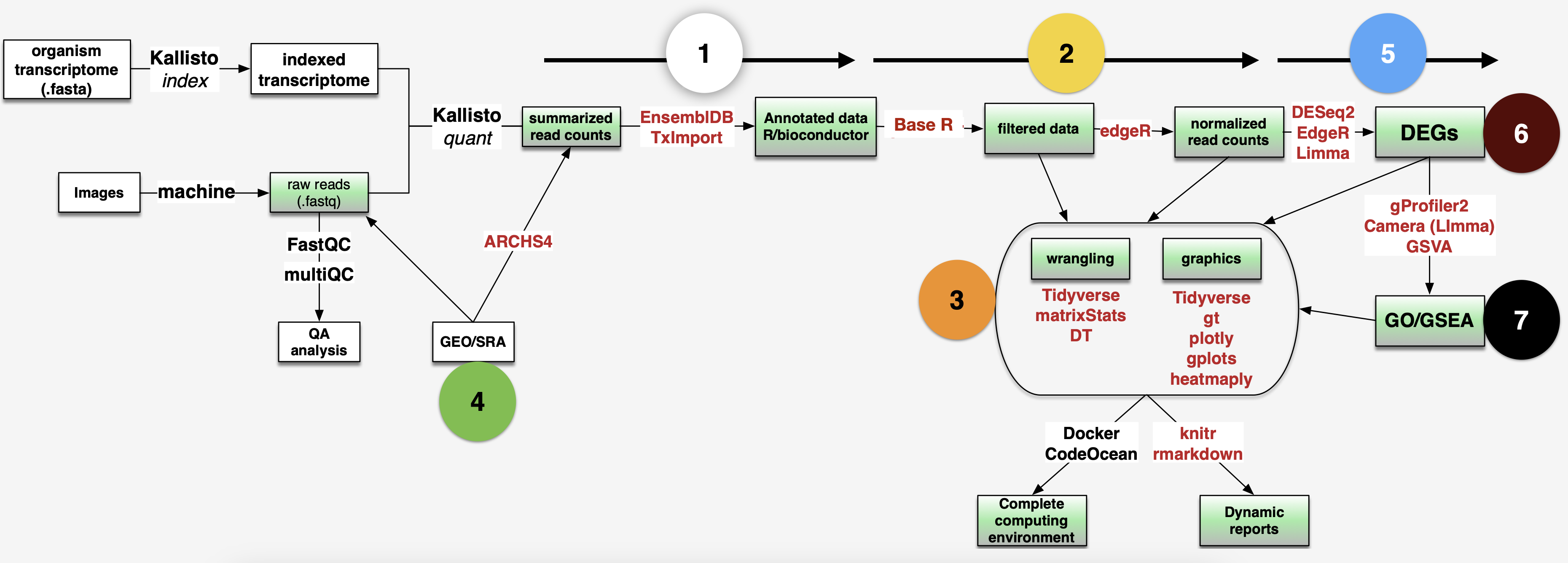
Step1: Check the quality of raw reads
### go to row reads folder
cd ~/../..DIY_Transcriptomics/data/fastq
### activate env
conda active rnaseq
### use fastqc to check the quality of fastq files
fastqc *.gz -t 4
Step2: Mapping reads with Kallisto pseudoaligment
Download reference transciptome files from here
Build an index from reference fasta file
kallisto index -i Homo_sapiens.GRCh38.cdna.all.index Homo_sapiens.GRCh38.cdna.all.fa.gz- Map reads to the indexed reference host transcriptome
- Summarize output with Multiqc in a single summary html
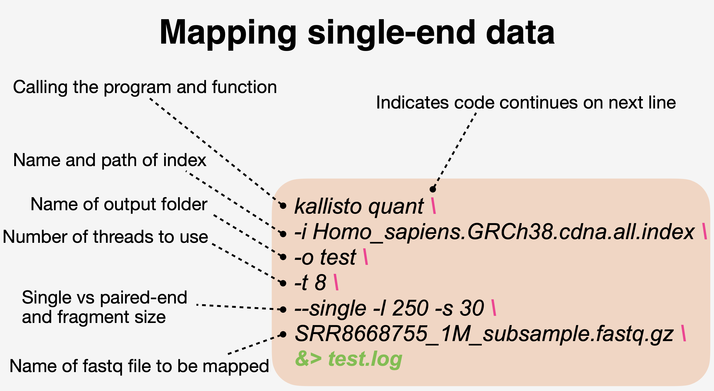
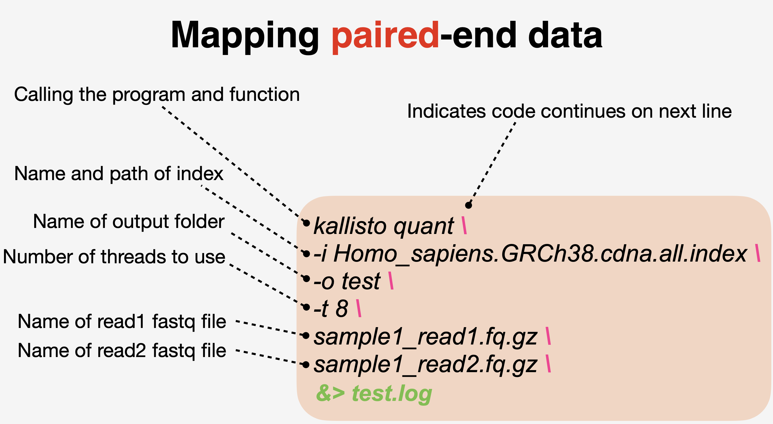
multiqc -d .### first the healthy subjects (HS)
kallisto quant -i Homo_sapiens.GRCh38.cdna.all.index -o HS01 -t 4 --single -l 250 -s 30 SRR8668755.fastq.gz &> HS01.log
kallisto quant -i Homo_sapiens.GRCh38.cdna.all.index -o HS02 -t 4 --single -l 250 -s 30 SRR8668756.fastq.gz &> HS02.log
kallisto quant -i Homo_sapiens.GRCh38.cdna.all.index -o HS03 -t 4 --single -l 250 -s 30 SRR8668757.fastq.gz &> HS03.log
kallisto quant -i Homo_sapiens.GRCh38.cdna.all.index -o HS04 -t 4 --single -l 250 -s 30 SRR8668758.fastq.gz &> HS04.log
kallisto quant -i Homo_sapiens.GRCh38.cdna.all.index -o HS05 -t 4 --single -l 250 -s 30 SRR8668759.fastq.gz &> HS05.log
### then the cutaneous leishmaniasis (CL) patients
kallisto quant -i Homo_sapiens.GRCh38.cdna.all.index -o CL08 -t 4 --single -l 250 -s 30 SRR8668769.fastq.gz &> CL08.log
kallisto quant -i Homo_sapiens.GRCh38.cdna.all.index -o CL10 -t 4 --single -l 250 -s 30 SRR8668771.fastq.gz &> CL10.log
kallisto quant -i Homo_sapiens.GRCh38.cdna.all.index -o CL11 -t 4 --single -l 250 -s 30 SRR8668772.fastq.gz &> CL11.log
kallisto quant -i Homo_sapiens.GRCh38.cdna.all.index -o CL12 -t 4 --single -l 250 -s 30 SRR8668773.fastq.gz &> CL12.log
kallisto quant -i Homo_sapiens.GRCh38.cdna.all.index -o CL13 -t 4 --single -l 250 -s 30 SRR8668774.fastq.gz &> CL13.log
### Summarize outputs
multiqc -d .Step3: Import data into R
Load packages
Import study design files
### load study design
targets <- read_tsv(
    here("learn", "DIY_Transcriptomics", "config", "studydesign.txt")
)
targets
## # A tibble: 10 × 3
##    sample sra_accession group
##    <chr>  <chr>         <chr>
##  1 HS01   SRR8668755    healthy
##  2 HS02   SRR8668756    healthy
##  3 HS03   SRR8668757    healthy
##  4 HS04   SRR8668758    healthy
##  5 HS05   SRR8668759    healthy
##  6 CL08   SRR8668769    disease
##  7 CL10   SRR8668771    disease
##  8 CL11   SRR8668772    disease
##  9 CL12   SRR8668773    disease
## 10 CL13   SRR8668774    disease

### create file paths for the abundance files
path <- file.path(
    "learn", "DIY_Transcriptomics", "data", "fastq", targets$sample, "abundance.tsv"
)
path
##  [1] "learn/DIY_Transcriptomics/data/fastq/HS01/abundance.tsv"
##  [2] "learn/DIY_Transcriptomics/data/fastq/HS02/abundance.tsv"
##  [3] "learn/DIY_Transcriptomics/data/fastq/HS03/abundance.tsv"
##  [4] "learn/DIY_Transcriptomics/data/fastq/HS04/abundance.tsv"
##  [5] "learn/DIY_Transcriptomics/data/fastq/HS05/abundance.tsv"
##  [6] "learn/DIY_Transcriptomics/data/fastq/CL08/abundance.tsv"
##  [7] "learn/DIY_Transcriptomics/data/fastq/CL10/abundance.tsv"
##  [8] "learn/DIY_Transcriptomics/data/fastq/CL11/abundance.tsv"
##  [9] "learn/DIY_Transcriptomics/data/fastq/CL12/abundance.tsv"
## [10] "learn/DIY_Transcriptomics/data/fastq/CL13/abundance.tsv"

### make sure path is correct
all(file.exists(path))
## [1] TRUE
Get organsim specific annotations
tx <- transcripts(
    EnsDb.Hsapiens.v86, columns = c("tx_id", "gene_name")
) |>
    as_tibble() |>
    ### need to change first column name to 'target_id'
    rename(target_id = tx_id)
tx
## # A tibble: 216,741 × 7
##    seqnames start   end width strand target_id       gene_name
##    <fct>    <int> <int> <int> <fct>  <chr>           <chr>
##  1 1        11869 14409  2541 +      ENST00000456328 DDX11L1
##  2 1        12010 13670  1661 +      ENST00000450305 DDX11L1
##  3 1        14404 29570 15167 -      ENST00000488147 WASH7P
##  4 1        17369 17436    68 -      ENST00000619216 MIR6859-1
##  5 1        29554 31097  1544 +      ENST00000473358 MIR1302-2
##  6 1        30267 31109   843 +      ENST00000469289 MIR1302-2
##  7 1        30366 30503   138 +      ENST00000607096 MIR1302-2
##  8 1        34554 36081  1528 -      ENST00000417324 FAM138A
##  9 1        35245 36073   829 -      ENST00000461467 FAM138A
## 10 1        52473 53312   840 +      ENST00000606857 OR4G4P
## # ℹ 216,731 more rows

### move transcrip ID the first column in the dataframe
tx <- select(tx, "target_id", "gene_name")
Load transcript counts
txi_gene <- tximport(
    path,
    type = "kallisto",
    tx2gene = tx,
    txOut = FALSE, # How does the result change if this =FALSE vs =TRUE?
    countsFromAbundance = "lengthScaledTPM",
    ignoreTxVersion = TRUE
)

### take a look at the type of object
class(txi_gene)
## [1] "list"
names(txi_gene)
## [1] "abundance"           "counts"              "length"
## [4] "countsFromAbundance"
Step4: Wrangling gene expression
### examine the data
tpm <- txi_gene$abundance
counts <- txi_gene$counts

### generate summary stats
tpm_stats <- transform(
    tpm,
    SD = rowSds(tpm),
    AVG = rowMeans(tpm),
    MED = rowMedians(tpm)
)

### look at the summary data
head(tpm_stats)
##                  X1          X2         X3           X4         X5          X6
## 5S_rRNA   0.0000000   0.0000000   0.000000   0.00000000   0.000000   0.0000000
## A1BG      6.3823340   6.7399420   3.842043   6.70710000   8.591181  14.6144150
## A1CF      0.0757872   0.0616752   0.214226   0.00859446   0.000000   0.0265036
## A2M     162.5622990 341.8312630 295.814803 261.47230600 169.453100 345.6983730
## A2ML1   109.6624900  80.6018680  90.356840  64.11152700  67.035650  52.5762220
## A2MP1     0.2237170   0.3143760   0.390022   0.15622800   0.122260   0.2700100
##                 X7          X8           X9         X10           SD
## 5S_rRNA   0.000000   0.0000000   0.00000000   0.0000000   0.00000000
## A1BG     18.182700  12.8662800  12.05296100   9.8268802   4.41172300
## A1CF      0.072777   0.1359934   0.03722713   0.0581254   0.06414927
## A2M     643.554440 341.8972850 324.80208900 415.9663840 135.78415021
## A2ML1     4.401309   5.1981760   1.75721000  15.1189910  39.78108982
## A2MP1     1.087410   0.7737610   0.68834900   0.6378640   0.31619850
##                  AVG         MED
## 5S_rRNA   0.00000000   0.0000000
## A1BG      9.98058361   9.2090306
## A1CF      0.06909094   0.0599003
## A2M     330.30523424 333.3166760
## A2ML1    49.08202830  58.3438745
## A2MP1     0.46639970   0.3521990

### visualize it using scatter plot
ggplot(tpm_stats, aes(x = SD, y = MED)) +
    geom_point(shape = 18, size = 2) +
    geom_smooth(method = lm) +
    geom_hex(show.legend = FALSE) +
    labs(
        y = "Median", x = "Standard deviation",
        title = "Transcripts per million (TPM)",
        subtitle = "unfiltered, non-normalized data",
        caption = "DIYtranscriptomics - Spring 2020"
    ) +
    theme_classic() +
    theme_dark() +
    theme_bw()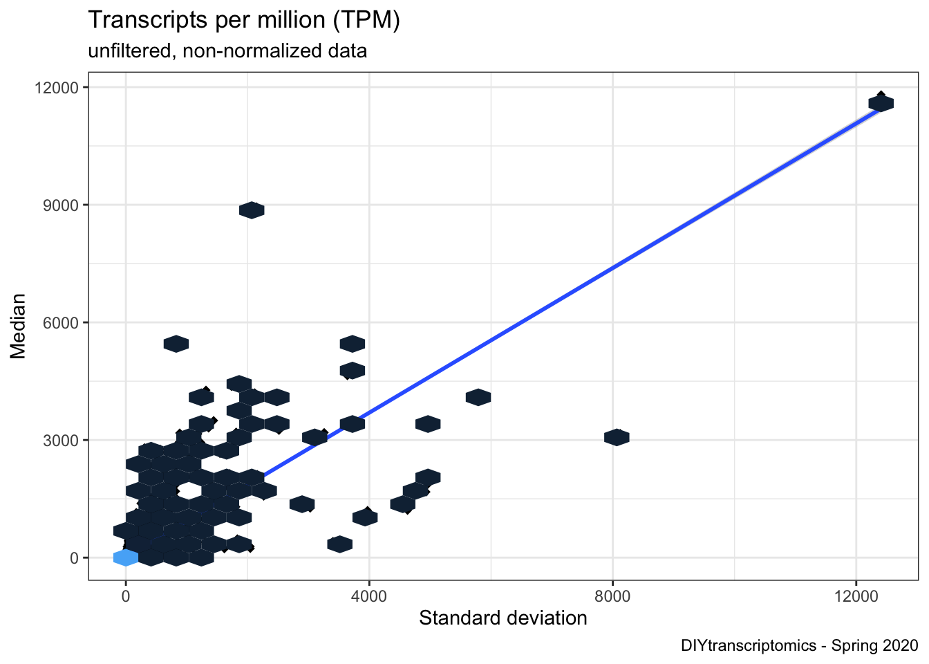
### capture sample labels from study design
sampleLabels <- targets$sample

### make DGElist from the counts
DGEList <- DGEList(txi_gene$counts)
DGEList
## An object of class "DGEList"
## $counts
##             Sample1     Sample2     Sample3     Sample4  Sample5     Sample6
## 5S_rRNA     0.00000     0.00000     0.00000    0.000000   0.0000     0.00000
## A1BG      184.19070   245.13169   101.73418   79.204797  13.3335   682.72256
## A1CF       22.94477    23.53171    59.50815    1.064719   0.0000    12.98875
## A2M     11901.13136 31538.08430 19870.31859 7832.900974 667.1460 40967.58721
## A2ML1   15162.86062 14045.04908 11463.06052 3627.335147 498.4618 11767.57706
##            Sample7     Sample8     Sample9    Sample10
## 5S_rRNA     0.0000     0.00000     0.00000     0.00000
## A1BG      391.5812   326.10430   397.97768   499.96534
## A1CF       16.4421    36.15938    12.89508    31.02343
## A2M     35158.3894 21982.61779 27205.95758 53686.20520
## A2ML1     454.1300   631.23251   277.98636  3685.37686
## 35366 more rows ...
##
## $samples
##          group lib.size norm.factors
## Sample1      1 42300696            1
## Sample2      1 51775632            1
## Sample3      1 40485664            1
## Sample4      1 16661634            1
## Sample5      1  2191577            1
## Sample6      1 55389922            1
## Sample7      1 28800520            1
## Sample8      1 31632164            1
## Sample9      1 39464569            1
## Sample10     1 67827185            1

### get counts per million
cpm <- cpm(DGEList)
colSums(cpm)
##  Sample1  Sample2  Sample3  Sample4  Sample5  Sample6  Sample7  Sample8
##    1e+06    1e+06    1e+06    1e+06    1e+06    1e+06    1e+06    1e+06
##  Sample9 Sample10
##    1e+06    1e+06

log2_cpm <- cpm(DGEList, log=TRUE)
### connvert data matrix to dataframe
log2_cpm_df <- as_tibble(log2_cpm, rownames = "geneID")
### add sample names
colnames(log2_cpm_df) <- c("geneID", sampleLabels)

### pivot from wide to long
log2_cpm_df_pivot <- pivot_longer(
  log2_cpm_df,
  cols = HS01:CL13,
  names_to = "samples",
  values_to = "expression"
)

p1 <- ggplot(
    log2_cpm_df_pivot,
    aes(x = samples, y = expression, fill = samples)
) +
    geom_violin(trim = FALSE, show.legend = FALSE) +
    stat_summary(fun = "median",
        geom = "point",
        shape = 95,
        size = 10,
        color = "black",
        show.legend = FALSE
    ) +
    labs(
        y = "log2 expression", x = "sample",
        title = "Log2 Counts per Million (CPM)",
        subtitle = "unfiltered, non-normalized",
        caption = paste0("produced on ", Sys.time())
    ) +
    theme_bw()
p1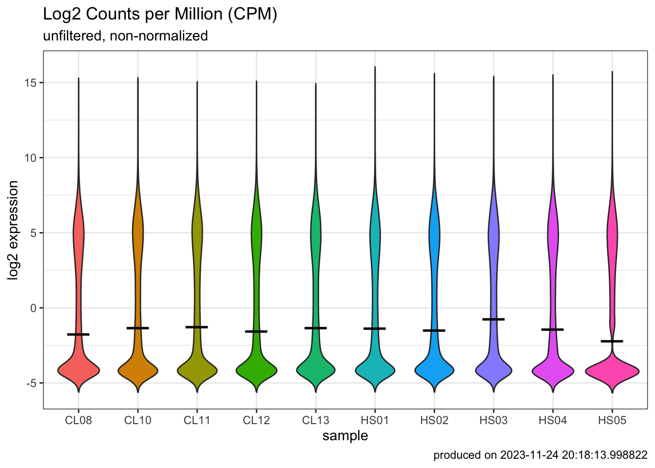
- How many genes or transcripts have no read counts at all?
### filter data
table(rowSums(DGEList$counts==0)==10)
##
## FALSE  TRUE
## 29373  5998

### how many genes had more than 1 CPM (TRUE) in at least 3 samples

### set cutoff
keepers <- rowSums(cpm>1) >= 5 # user defined
DGEList_filtered <- DGEList[keepers, ]

log2_cpm_filtered <- cpm(DGEList_filtered, log=TRUE)
log2_cpm_filtered_df <- as_tibble(log2_cpm_filtered, rownames = "geneID")
colnames(log2_cpm_filtered_df) <- c("geneID", sampleLabels)
log2_cpm_filtered_df_pivot <- pivot_longer(
    log2_cpm_filtered_df,
    cols = HS01:CL13,
    names_to = "samples",
    values_to = "expression"
)

p2 <- ggplot(
    log2_cpm_filtered_df_pivot,
    aes(x = samples, y = expression, fill = samples)
) +
    geom_violin(trim = FALSE, show.legend = FALSE) +
    stat_summary(
        fun = "median",
        geom = "point",
        shape = 95,
        size = 10,
        color = "black",
        show.legend = FALSE
    ) +
    labs(y = "log2 expression", x = "sample",
        title = "Log2 Counts per Million (CPM)",
        subtitle = "filtered, non-normalized",
        caption = paste0("produced on ", Sys.time())) +
    theme_bw()

p2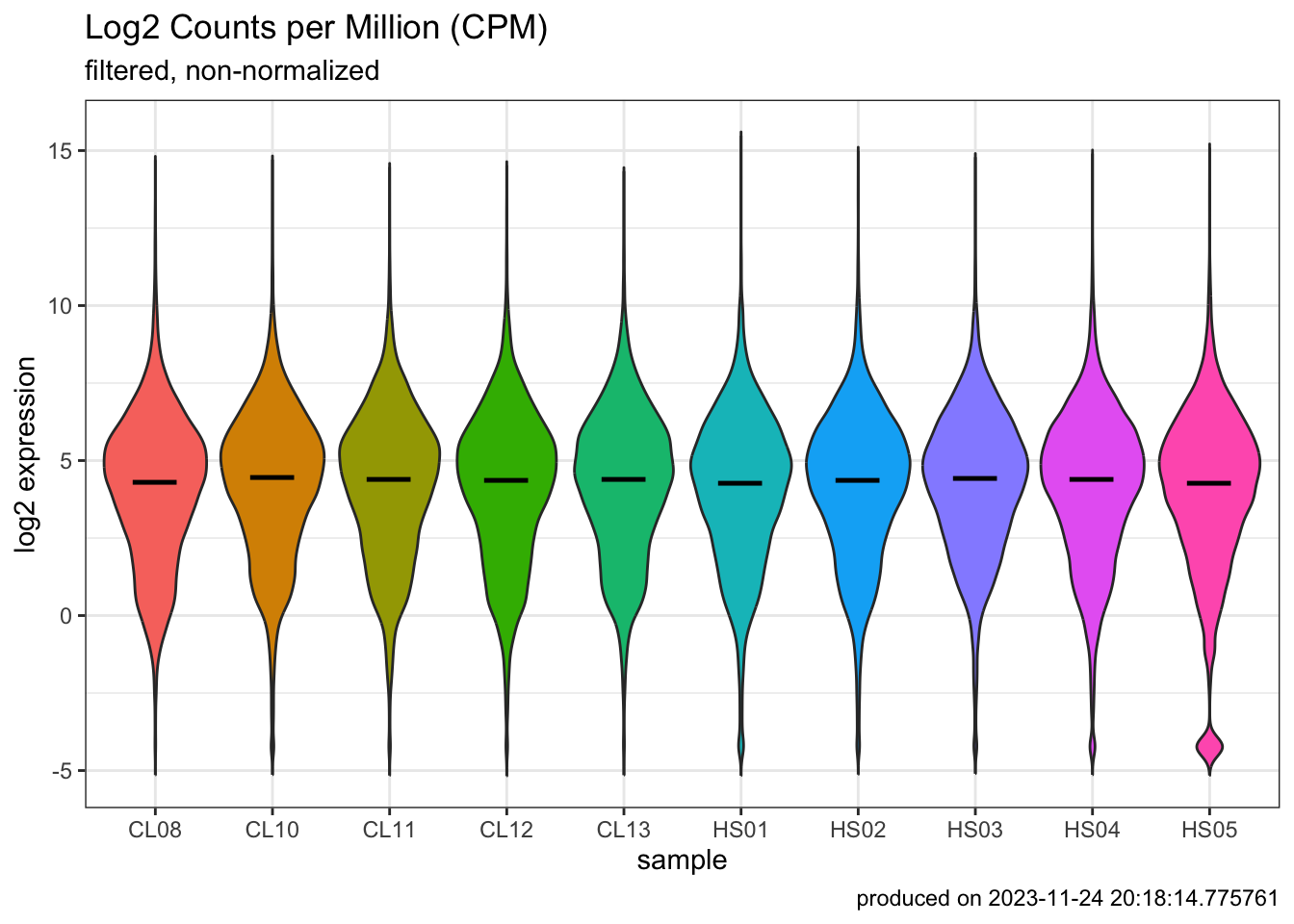
### normalize data
DGEList_filtered_norm <- calcNormFactors(
DGEList_filtered, method = "TMM"
)
log2_cpm_filtered_norm <- cpm(
DGEList_filtered_norm, log = TRUE
)
log2_cpm_filtered_norm_df <- as_tibble(
log2_cpm_filtered_norm, rownames = "geneID"
)
colnames(log2_cpm_filtered_norm_df) <- c("geneID", sampleLabels)
log2_cpm_filtered_norm_df_pivot <- pivot_longer(
log2_cpm_filtered_norm_df,
cols = HS01:CL13,
names_to = "samples",
values_to = "expression"
)
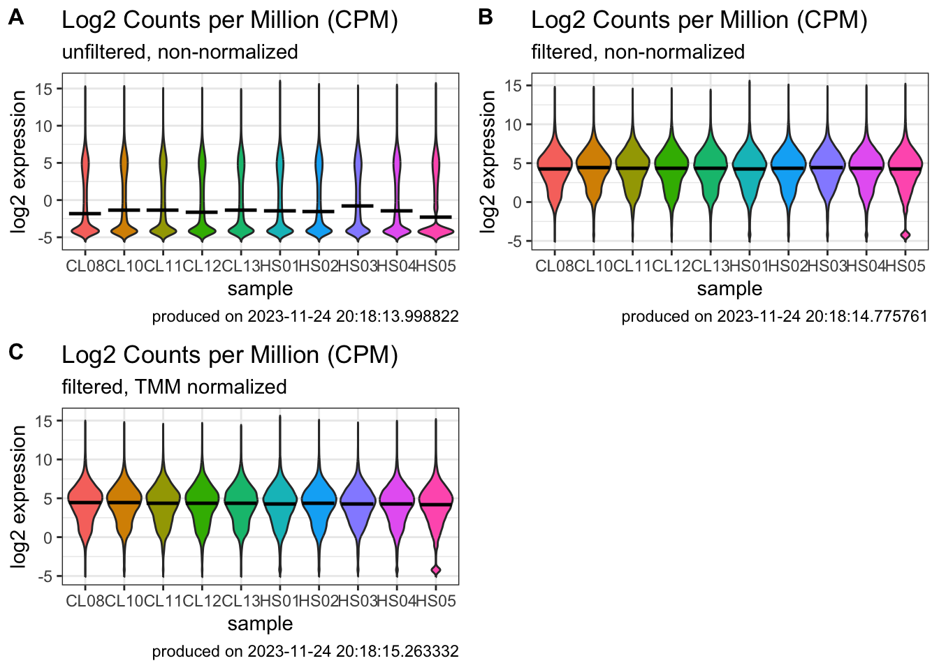
p3 <- ggplot(
log2_cpm_filtered_norm_df_pivot,
aes(x = samples, y = expression, fill = samples)
) +
geom_violin(trim = FALSE, show.legend = FALSE) +
stat_summary(
fun = "median",
geom = "point",
shape = 95,
size = 10,
color = "black",
show.legend = FALSE
) +
labs(
y = "log2 expression", x = "sample",
title = "Log2 Counts per Million (CPM)",
subtitle = "filtered, TMM normalized",
caption = paste0("produced on ", Sys.time())
) +
theme_bw()
### combine plots
plot_grid(
p1, p2, p3,
labels = c('A', 'B', 'C'),
label_size = 12
)
Step5: Data exploration with multivariate analysis
### Identify variables of interest in study design file
group <- targets$group
group <- factor(group)
group
##  [1] healthy healthy healthy healthy healthy disease disease disease disease
## [10] disease
## Levels: disease healthy
Hierarchical clustering
### calculate distance  methods (e.g. switch from 'maximum' to 'euclidean')
distance <- dist(
    t(log2_cpm_filtered_norm), method = "maximum"
)
### other distance methods are "euclidean", maximum", "manhattan", "canberra", "binary" or "minkowski"

clusters <- hclust(distance, method = "average")
### other agglomeration methods are "ward.D", "ward.D2", "single", "complete", "average", "mcquitty", "median", or "centroid"
plot(clusters, labels=sampleLabels)
Principal compoent analysis
pca_res <- prcomp(
    t(log2_cpm_filtered_norm),
    scale. = FALSE, retx = TRUE
)


### prints variance summary for all principal components.
summary(pca_res)
## Importance of components:
##                             PC1     PC2      PC3      PC4      PC5      PC6
## Standard deviation     113.9821 49.8074 33.42376 27.08082 26.40296 22.23750
## Proportion of Variance   0.6656  0.1271  0.05723  0.03757  0.03571  0.02533
## Cumulative Proportion    0.6656  0.7927  0.84993  0.88750  0.92322  0.94855
##                             PC7      PC8      PC9      PC10
## Standard deviation     20.50645 17.71945 16.42366 1.816e-13
## Proportion of Variance  0.02154  0.01609  0.01382 0.000e+00
## Cumulative Proportion   0.97010  0.98618  1.00000 1.000e+00

### look at the PCA result (pca.res)
ls(pca_res)
## [1] "center"   "rotation" "scale"    "sdev"     "x"

### $rotation shows you how much each gene influenced each PC (called 'scores')
head(pca_res$rotation)
##                 PC1          PC2           PC3          PC4           PC5
## A1BG    0.006058601 -0.005265865  0.0030322868  0.008759217  0.0021903806
## A2M     0.004897345  0.002459393 -0.0029437295  0.010128989  0.0010754828
## A2ML1  -0.015426376  0.002131922  0.0236833694  0.012776801  0.0151330784
## A2MP1   0.008361769  0.005416383 -0.0080073403 -0.004989098  0.0019137300
## A4GALT -0.004861196 -0.010071400 -0.0040747825  0.004365382 -0.0073287027
## AAAS    0.002247684 -0.005546829 -0.0003891962  0.005401109 -0.0008667994
##                 PC6           PC7         PC8          PC9        PC10
## A1BG    0.002600255  1.165903e-02 0.002109927  0.006017461 -0.62642253
## A2M    -0.003082754 -2.988929e-03 0.007583352 -0.002958490 -0.07649096
## A2ML1  -0.013272183 -1.389944e-02 0.008501332  0.020687796  0.29435235
## A2MP1  -0.002415560  1.626299e-03 0.011281299 -0.005577339 -0.50451276
## A4GALT -0.009698589  6.199904e-05 0.012467687  0.004110126 -0.31572438
## AAAS    0.006991981  3.783003e-03 0.004628266  0.003568768 -0.14061416

### 'x' shows you how much each sample influenced each PC (called 'loadings')
pca_res$x
##                 PC1          PC2        PC3        PC4         PC5        PC6
## Sample1  -116.29139   38.2334807  21.154790 -31.204512  24.3342557  -5.032445
## Sample2   -98.08443   28.5182187   6.488451  20.455248 -24.7150117  -5.625522
## Sample3   -98.57599   46.3377421 -21.880766 -22.638077  26.9619112   8.312240
## Sample4  -102.83232   27.1997919 -10.521681  36.884584 -34.6489813  11.837625
## Sample5  -119.48548 -130.0448432  -8.771308  -8.078419   0.7747427  -2.609032
## Sample6    76.83934  -13.0282654  65.541177  34.668976  32.4966464   9.756467
## Sample7   114.80802    0.9427947 -66.411954  27.226075  30.8708143  -6.756527
## Sample8   122.14072   -0.8992447  -2.600281 -31.000051 -26.0328136  19.278692
## Sample9   129.23356   -4.8764679   3.983424 -16.285254 -13.4446636  25.667565
## Sample10   92.24799    7.6167930  13.018146 -10.028570 -16.5969001 -54.829063
##                 PC7         PC8         PC9          PC10
## Sample1   37.289161  -8.2755495   9.2338103  6.432316e-13
## Sample2    9.263960  37.6085903 -14.4523481  7.064106e-14
## Sample3  -40.584484   0.6580365  -8.3486393  3.455381e-13
## Sample4   -3.089166 -28.1333136  11.4331050 -5.619926e-14
## Sample5   -2.014396  -0.2124505  -0.6860841 -1.205842e-13
## Sample6  -10.563273   2.1965073   5.3204553 -6.485607e-14
## Sample7   15.193876   4.0838551   4.1812220 -2.588419e-13
## Sample8   -5.936520  15.6564254  28.6671255 -1.908206e-13
## Sample9   11.836127 -13.5624080 -32.5109827 -3.271781e-13
## Sample10 -11.395285 -10.0196929  -2.8376640  1.788202e-13

### A screeplot is a standard way to view eigenvalues for each PCA
screeplot(pca_res) 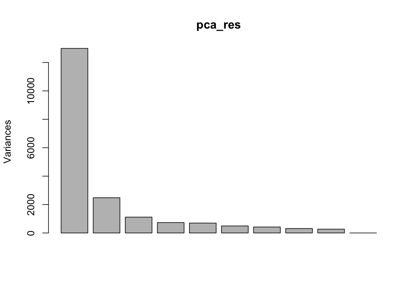
- Can we figure out the identify of outlier?
### visualize PCA result
pca_res_df <- as_tibble(pca_res$x) |>
  bind_cols(targets) |>
  mutate(group = factor(group))
pca_plot1 <- pca_res_df |>
    ggplot(
        aes(x = PC1, y = PC2, label = sample, color = group)
    ) +
    geom_point(size = 4) +
    stat_ellipse() +
    xlab(paste0("PC1 (", pc_per[1], "%", ")")) +
    ylab(paste0("PC2 (", pc_per[2], "%", ")")) +
    labs(title = "PCA plot",
        caption = paste0("produced on ", Sys.time())) +
    coord_fixed() +
    theme_bw()

pca_plot1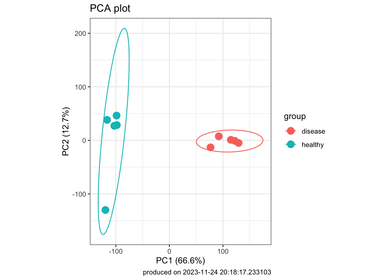
- Another way to view PCA laodings to understand impact of each sample on each pricipal component
pca_res_df <- pca_res$x[, 1:4] |>
    as_tibble() |>
    add_column(
        sample = sampleLabels,
        group = group
    )
### dataframe to be pivoted
pca_pivot <- pivot_longer(
  pca_res_df,
  cols = PC1:PC4,
  names_to = "PC",
  values_to = "loadings"
)
### plot
pca_plot2 <- ggplot(pca_pivot) +
    aes(x = sample, y = loadings, fill = group) +
    geom_bar(stat = "identity") +
    facet_wrap(~PC) +
    labs(
        title = "PCA 'small multiples' plot",
        caption = paste0("produced on ", Sys.time())
    ) +
    theme_bw() +
    coord_flip()
pca_plot2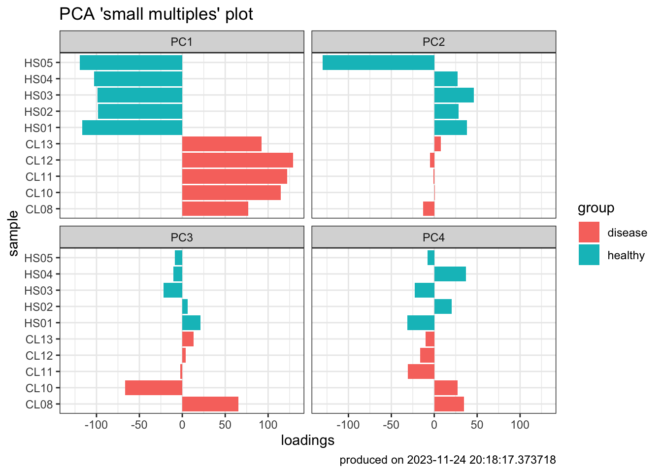
### combine plot
# plot_grid(pca_plot1, pca_plot2)
# make columns comparing each of the averages above that you're interested in
mydata_df <- mutate(
log2_cpm_filtered_norm_df,
healthy.AVG = (HS01 + HS02 + HS03 + HS04 + HS05)/5,
disease.AVG = (CL08 + CL10 + CL11 + CL12 + CL13)/5,
LogFC = (disease.AVG - healthy.AVG)
) |>
mutate_if(is.numeric, round, 2)
### sort data
mydata_sort <- mydata_df |>
arrange(desc(LogFC)) |>
select(geneID, LogFC)
mydata_sort
## # A tibble: 15,765 × 2
## geneID LogFC
## <chr> <dbl>
## 1 IGLC3 10.6
## 2 MMP1 10.4
## 3 IGKV1-5 10.2
## 4 IGLV3-1 9.96
## 5 IGLV3-19 9.9
## 6 IGLC1 9.88
## 7 IGKV1D-39 9.87
## 8 IGLL5 9.85
## 9 IGKV1D-33 9.83
## 10 IGLV2-8 9.65
## # ℹ 15,755 more rows
### filter data
mydata_filter <- mydata_df |>
filter(
geneID == "MMP1" | geneID == "GZMB" | geneID == "IL1B" | geneID == "GNLY" | geneID == "IFNG"
| geneID == "CCL4" | geneID == "PRF1" | geneID == "APOBEC3A" | geneID == "UNC13A"
) |>
select(geneID, healthy.AVG, disease.AVG, LogFC) |>
arrange(desc(LogFC))
mydata_filter
## # A tibble: 9 × 4
## geneID healthy.AVG disease.AVG LogFC
## <chr> <dbl> <dbl> <dbl>
## 1 MMP1 1.44 11.9 10.4
## 2 IFNG -3.65 4.42 8.07
## 3 CCL4 -1.75 6.14 7.89
## 4 GZMB -0.58 6.47 7.05
## 5 GNLY 0.98 7.17 6.19
## 6 IL1B 0.63 6.48 5.85
## 7 PRF1 1.03 6.64 5.61
## 8 APOBEC3A 0.27 5.6 5.33
## 9 UNC13A -0.78 1.95 2.73### Produce publication-quality tables using `gt` package
mydata_filter |>
gt() |>
fmt_number(columns = 2:4, decimals = 1) |>
tab_header(
title = md("**Regulators of skin pathogenesis**"),
subtitle = md("*during cutaneous leishmaniasis*")
) |>
tab_footnote(
footnote = "Deletion or blockaid ameliorates disease in mice",
locations = cells_body(columns = geneID, rows = c(6, 7))
) |>
tab_footnote(
footnote = "Associated with treatment failure in multiple studies",
locations = cells_body(columns = geneID, rows = c(2:9))
) |>
tab_footnote(
footnote = "Implicated in parasite control",
locations = cells_body(columns = geneID, rows = c(2))
) |>
tab_source_note(
source_note = md("Reference: Amorim *et al*., (2019). DOI: 10.1126/scitranslmed.aar3619")
)| Regulators of skin pathogenesis | |||
| during cutaneous leishmaniasis | |||
| geneID | healthy.AVG | disease.AVG | LogFC |
|---|---|---|---|
| MMP1 | 1.4 | 11.9 | 10.4 |
| IFNG1,2 | −3.6 | 4.4 | 8.1 |
| CCL41 | −1.8 | 6.1 | 7.9 |
| GZMB1 | −0.6 | 6.5 | 7.0 |
| GNLY1 | 1.0 | 7.2 | 6.2 |
| IL1B3,1 | 0.6 | 6.5 | 5.8 |
| PRF13,1 | 1.0 | 6.6 | 5.6 |
| APOBEC3A1 | 0.3 | 5.6 | 5.3 |
| UNC13A1 | −0.8 | 1.9 | 2.7 |
| Reference: Amorim et al., (2019). DOI: 10.1126/scitranslmed.aar3619 | |||
| 1 Associated with treatment failure in multiple studies | |||
| 2 Implicated in parasite control | |||
| 3 Deletion or blockaid ameliorates disease in mice | |||
- Make an interactive table using the
DTpackage
# datatable(
#     mydata_df[, c(1, 12:14)],
#     extensions = c('KeyTable', "FixedHeader"),
#     filter = 'top',
#     options = list(keys = TRUE,
#         searchHighlight = TRUE,
#         pageLength = 10,
#         # dom = "Blfrtip",
#         # buttons = c("copy", "csv", "excel"),
#         lengthMenu = c("10", "25", "50", "100"))
# )- Make an interactive scatter plot with
plotly
myplot <- ggplot(mydata_df) +
  aes(x=healthy.AVG, y=disease.AVG,
      text = paste("Symbol:", geneID)) +
  geom_point(shape=16, size=1) +
  ggtitle("disease vs. healthy") +
  theme_bw()

myplot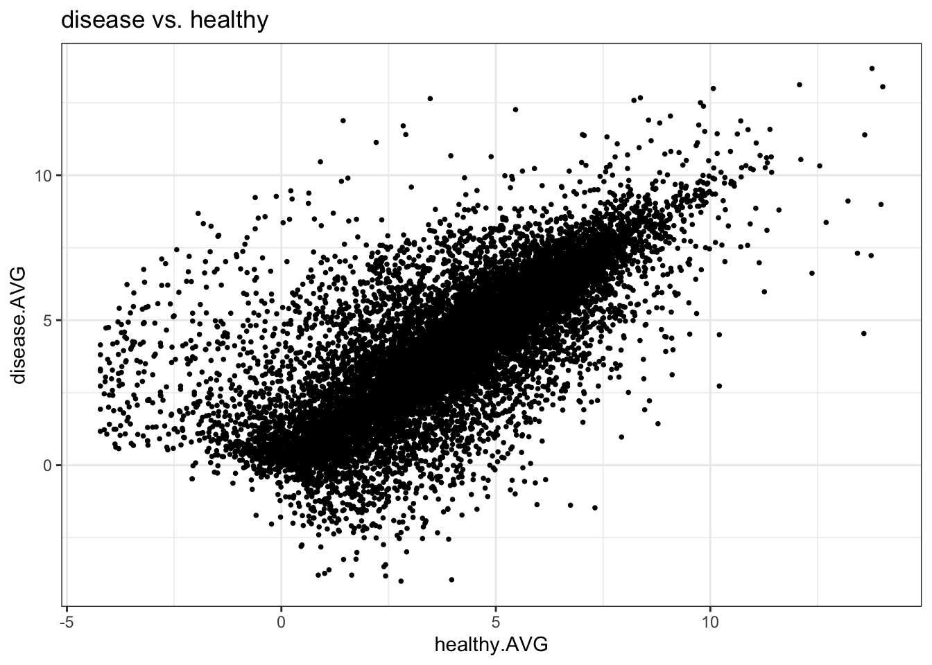
# ggplotly(myplot)Step6: Differential gene expression
Set up design matrix
group <- factor(targets$group)
design <- model.matrix(~0 + group)
colnames(design) <- levels(group)

# NOTE: if you need a paired analysis (a.k.a.'blocking' design) or have a batch effect, the following design is useful
# design <- model.matrix(~block + treatment)
# this is just an example. 'block' and 'treatment' would need to be objects in your environment
Model mean-variance trend and fit linear model to data
### Use VOOM function from Limma package to model the mean-variance relationship
head(DGEList_filtered_norm)
## An object of class "DGEList"
## $counts
##            Sample1     Sample2     Sample3    Sample4     Sample5     Sample6
## A1BG     184.19070   245.13169   101.73418   79.20480  13.3334957   682.72256
## A2M    11901.13136 31538.08430 19870.31859 7832.90097 667.1460374 40967.58721
## A2ML1  15162.86062 14045.04908 11463.06052 3627.33515 498.4617540 11767.57706
## A2MP1     29.31478    51.91491    46.89141    8.37674   0.8615391    57.27197
## A4GALT   128.32345   355.39448   131.42493   75.43359  30.6454026   112.79123
## AAAS     269.07806   457.62142   257.49394  147.56154  27.9749726   636.62246
##            Sample7     Sample8    Sample9   Sample10
## A1BG     391.58119   326.10430   397.9777   499.9653
## A2M    35158.38935 21982.61779 27205.9576 53686.2052
## A2ML1    454.12997   631.23251   277.9864  3685.3769
## A2MP1    106.33010    89.04506   103.1984   147.3506
## A4GALT    87.64872    88.03357    62.6173   230.0622
## AAAS     382.02897   412.70476   446.8081   509.4904
##
## $samples
##          group lib.size norm.factors
## Sample1      1 42300696    0.9838341
## Sample2      1 51775632    1.0056785
## Sample3      1 40485664    1.1055948
## Sample4      1 16661634    1.0332639
## Sample5      1  2191577    1.0154852
## Sample6      1 55389922    0.8810033
## Sample7      1 28800520    1.0117840
## Sample8      1 31632164    1.0093077
## Sample9      1 39464569    0.9639270
## Sample10     1 67827185    1.0046274
v_DEGList_filtered_norm <- voom(DGEList_filtered_norm, design, plot = TRUE)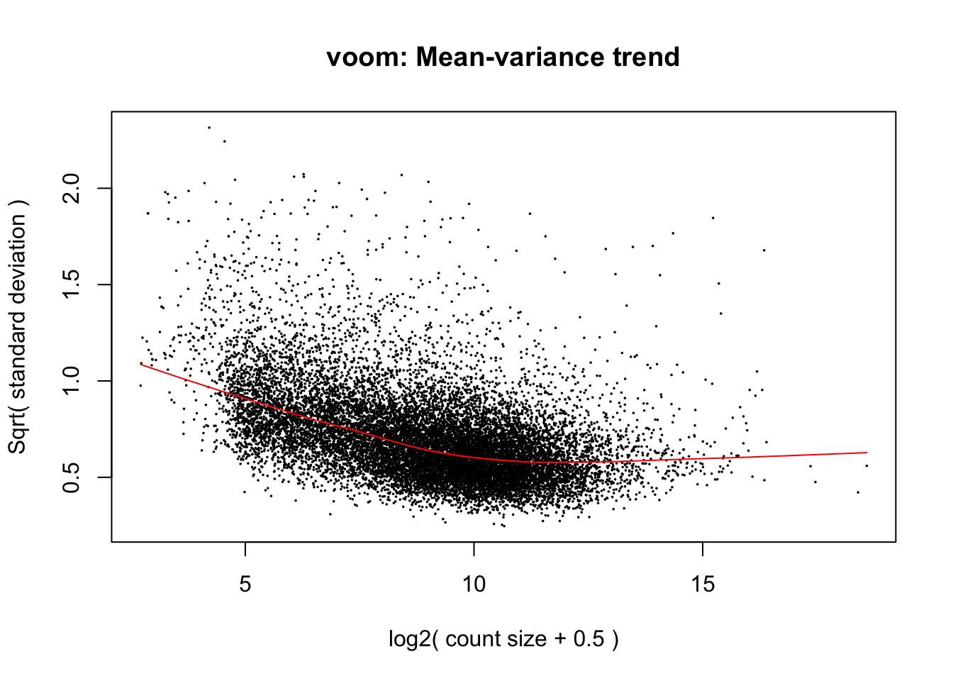
# fit a linear model to your data
fit <- lmFit(v_DEGList_filtered_norm, design)

### contrast matrix
contrast_matrix <- makeContrasts(infection = disease - healthy,
                                 levels=design)
### extract the linear model fit
fits <- contrasts.fit(fit, contrast_matrix)

### get bayesian stats for the linear model fit
ebFit <- eBayes(fits)

#write.fit(ebFit, file="lmfit_results.txt")

### top table to view DEGs
TopHits <- topTable(ebFit, adjust ="BH", coef=1, number=40000, sort.by="logFC")

### convert to a tibble
TopHits_df <- TopHits |>
  as_tibble(rownames = "geneID")

TopHits_df
## # A tibble: 15,765 × 7
##    geneID    logFC AveExpr     t      P.Value  adj.P.Val     B
##    <chr>     <dbl>   <dbl> <dbl>        <dbl>      <dbl> <dbl>
##  1 MMP1      10.8    6.65  13.4  0.0000000182 0.00000123 10.0
##  2 IGLC3     10.3    3.49   7.50 0.00000815   0.0000778   4.06
##  3 IGKV1D-33 10.2    1.12   9.29 0.000000913  0.0000160   6.11
##  4 IGKV2D-28 10.1    0.898  9.50 0.000000723  0.0000137   6.32
##  5 IGLV3-25  10.0    0.242  6.89 0.0000186    0.000147    3.27
##  6 IGLV3-1   10.0    1.75  11.8  0.0000000715 0.00000281  8.36
##  7 IGKV1-5    9.93   3.36  13.8  0.0000000124 0.00000101 10.0
##  8 IGHV1-3    9.89   0.447  6.24 0.0000468    0.000302    2.37
##  9 IGLV3-19   9.84   2.18   6.93 0.0000175    0.000140    3.33
## 10 IGHV3-21   9.80   1.42   9.00 0.00000128   0.0000200   5.80
## # ℹ 15,755 more rows
Limma outputs
- TopTable (from Limma) outputs a few different stats:
- logFC, AveExpr, and P.Value should be self-explanatory
- adj.P.Val is your adjusted P value, also known as an FDR (if BH method was used for multiple testing correction)
- B statistic is the log-odds that that gene is differentially expressed. If B = 1.5, then log odds is e^1.5, where e is euler’s constant (approx. 2.718). So, the odds of differential expression os about 4.8 to 1
- t statistic is ratio of the logFC to the standard error (where the error has been moderated across all genes…because of Bayesian approach)
### volcano plot
vplot <- TopHits_df |>
    ggplot(
        aes(y = -log10(adj.P.Val), x = logFC, text = paste("Symbol:", geneID))
    ) +
    geom_point(size = 2) +
    geom_hline(yintercept = -log10(0.01), linetype = "longdash", colour = "grey", linewidth = 1) +
    geom_vline(xintercept = 1, linetype = "longdash", colour = "#BE684D", linewidth = 1) +
    geom_vline(xintercept = -1, linetype = "longdash", colour = "#2C467A", linewidth = 1) +
    # annotate("rect", xmin = 1, xmax = 12, ymin = -log10(0.01), ymax = 7.5, alpha=.2, fill="#BE684D") +
    # annotate("rect", xmin = -1, xmax = -12, ymin = -log10(0.01), ymax = 7.5, alpha=.2, fill="#2C467A") +
    labs(title = "Volcano plot",
        subtitle = "Cutaneous leishmaniasis",
        caption = paste0("produced on ", Sys.time())) +
    theme_bw()

vplot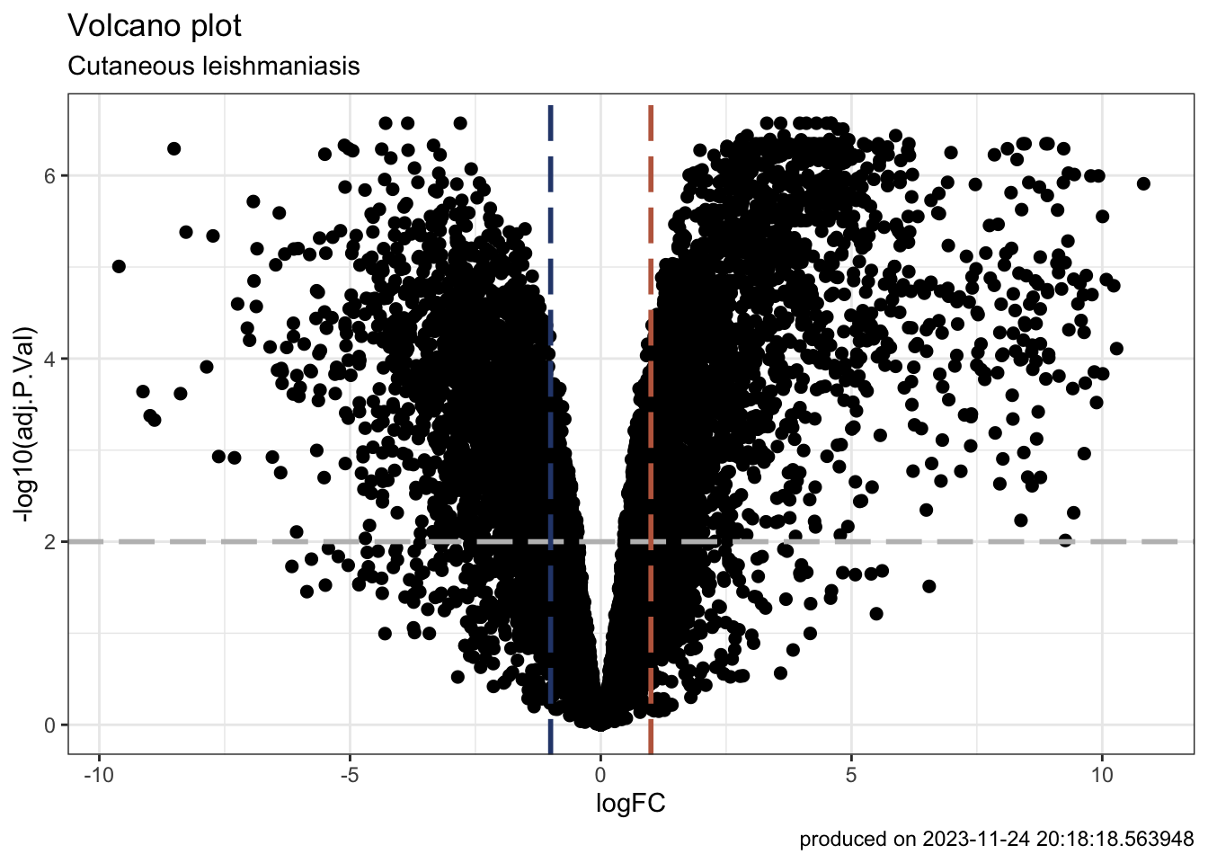
### pull out DEGs and make venn diagram
results <- decideTests(
    ebFit, method = "global", adjust.method = "BH", p.value = 0.01, lfc = 2
)
head(results)
## TestResults matrix
##         Contrasts
##          infection
##   A1BG           0
##   A2M            0
##   A2ML1         -1
##   A2MP1          0
##   A4GALT         0
##   AAAS           0
summary(results)
##        infection
## Down        1012
## NotSig     13446
## Up          1307
vennDiagram(results, include="up")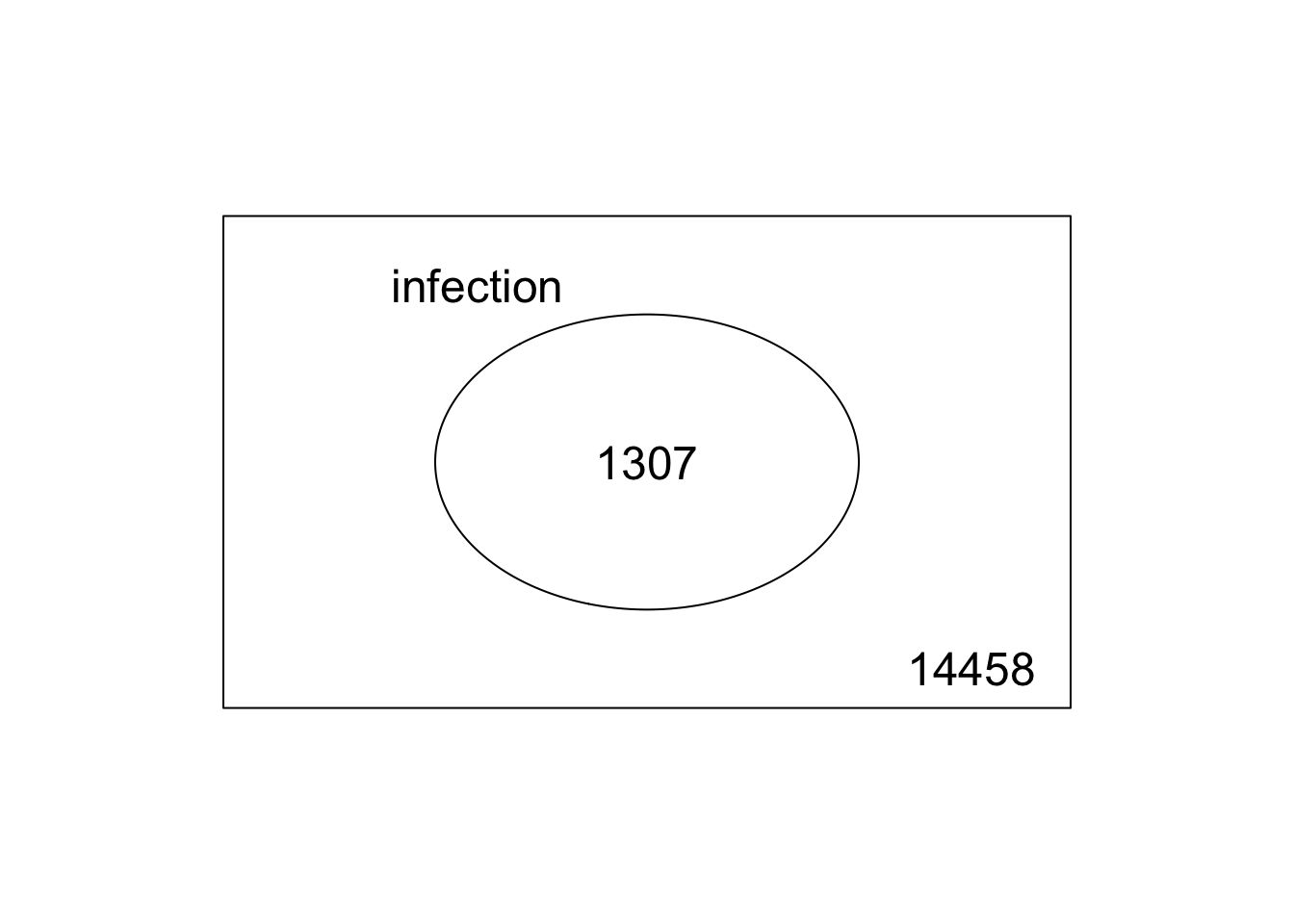
### retrieve expression data for DEGs
head(v_DEGList_filtered_norm$E)
## Sample1 Sample2 Sample3 Sample4 Sample5 Sample6
## A1BG 2.1498709 2.237982296 1.19157184 2.2109278 2.6359548 3.8074408
## A2M 8.1597752 9.242459704 8.79420169 8.8297563 8.2288005 9.7134419
## A2ML1 8.5092054 8.075454826 8.00060559 7.7192264 7.8086463 7.9138199
## A2MP1 -0.4811408 0.009534871 0.08239155 -0.9556369 -0.7089007 0.2435267
## A4GALT 1.6301549 2.772935178 1.55941146 2.1409994 3.8068082 1.2151214
## AAAS 2.6954627 3.137215647 2.52703139 3.1043863 3.6774835 3.7066558
## Sample7 Sample8 Sample9 Sample10
## A1BG 3.750084 3.354713 3.3888732 2.876674
## A2M 10.236678 9.427422 9.4821796 9.621825
## A2ML1 3.963625 4.306483 2.8719810 5.757340
## A2MP1 1.874250 1.487855 1.4467684 1.117544
## A4GALT 1.596943 1.471466 0.7304817 1.758560
## AAAS 3.714501 3.694027 3.5556433 2.903874
colnames(v_DEGList_filtered_norm$E) <- sampleLabels
diffGenes <- v_DEGList_filtered_norm$E[results[,1] !=0,]
head(diffGenes)
## HS01 HS02 HS03 HS04 HS05 CL08 CL10
## A2ML1 8.509205 8.075455 8.000606 7.719226 7.808646 7.913820 3.9636246
## AADAC 3.783598 3.145125 3.421001 3.846583 4.124090 2.241617 -3.5057299
## AADACL2 6.884775 7.025967 6.096531 6.700546 6.104662 5.215819 -5.8649243
## AARD 2.817882 1.719728 2.562007 2.090062 2.784928 1.028134 0.2785801
## ABCA10 4.429922 4.330043 6.261231 3.871370 2.785400 2.261820 2.9336235
## ABCA12 8.609129 7.810834 7.884251 7.603805 7.963791 7.338358 3.3247149
## CL11 CL12 CL13
## A2ML1 4.3064835 2.8719810 5.7573398
## AADAC 0.1777154 -0.9997370 -0.5843452
## AADACL2 2.9288016 2.0251967 3.5424241
## AARD 0.2142361 -0.4255113 0.1288021
## ABCA10 2.4838643 2.4430992 0.6882190
## ABCA12 5.2844659 4.7055495 6.6999992
dim(diffGenes)
## [1] 2319 10
#convert DEGs to a dataframe using as_tibble
diffGenes_df <- as_tibble(diffGenes, rownames = "geneID")
### create interactive tables to display DEGs
# datatable(diffGenes_df,
# extensions = c('KeyTable', "FixedHeader"),
# caption = 'Table 1: DEGs in cutaneous leishmaniasis',
# options = list(keys = TRUE, searchHighlight = TRUE, pageLength = 10, lengthMenu = c("10", "25", "50", "100"))) |>
# formatRound(columns=c(2:11), digits=2)
### write DEGs to a file
# write_tsv(diffGenes_df, "DiffGenes.txt")
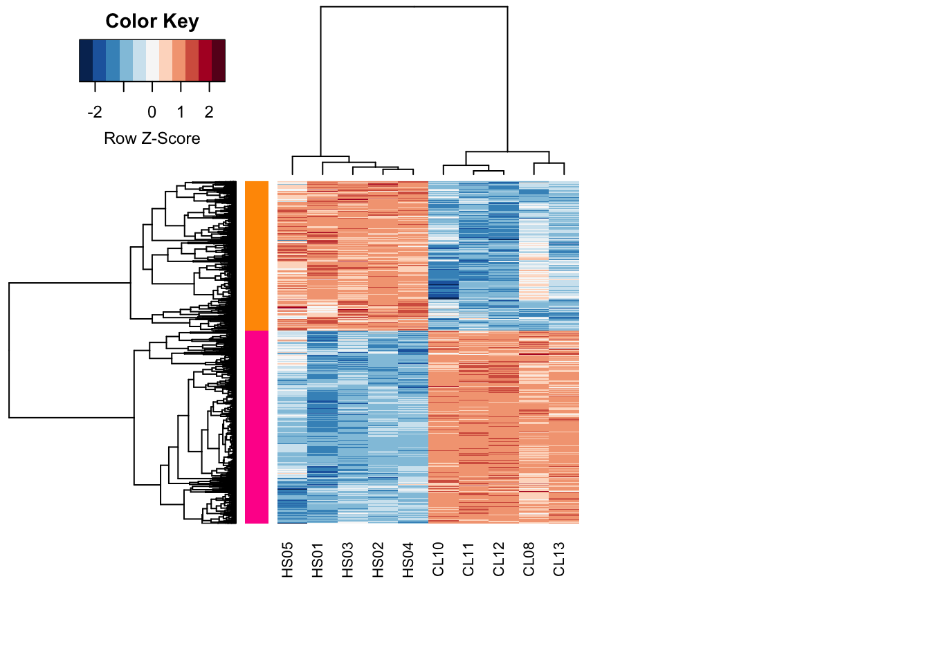
#NOTE: this .txt file can be directly used for input into other clustering or network analysis tools (e.g., String, Clust (https://github.com/BaselAbujamous/clust, etc.)Step7: Module identification
heatcolors <- rev(brewer.pal(name="RdBu", n=11))

#cluster rows by pearson correlation
clustRows <- hclust(
  as.dist(1-cor(t(diffGenes), method="pearson")),
  method="complete"
)
#cluster columns by pearson correlation
clustColumns <- hclust(
  as.dist(1-cor(diffGenes, method="spearman")),
  method="complete"
  )

module_assign <- cutree(clustRows, k=2)

module_color <- rainbow(length(unique(module_assign)), start=0.1, end=0.9)

module_color <- module_color[as.vector(module_assign)]

heatmap.2(
    diffGenes,
    Rowv = as.dendrogram(clustRows),
    Colv = as.dendrogram(clustColumns),
    RowSideColors = module_color,
    col = heatcolors, scale = 'row', labRow = NA,
    density.info = "none", trace = "none",
    cexRow = 1, cexCol = 1, margins = c(8, 20)
)
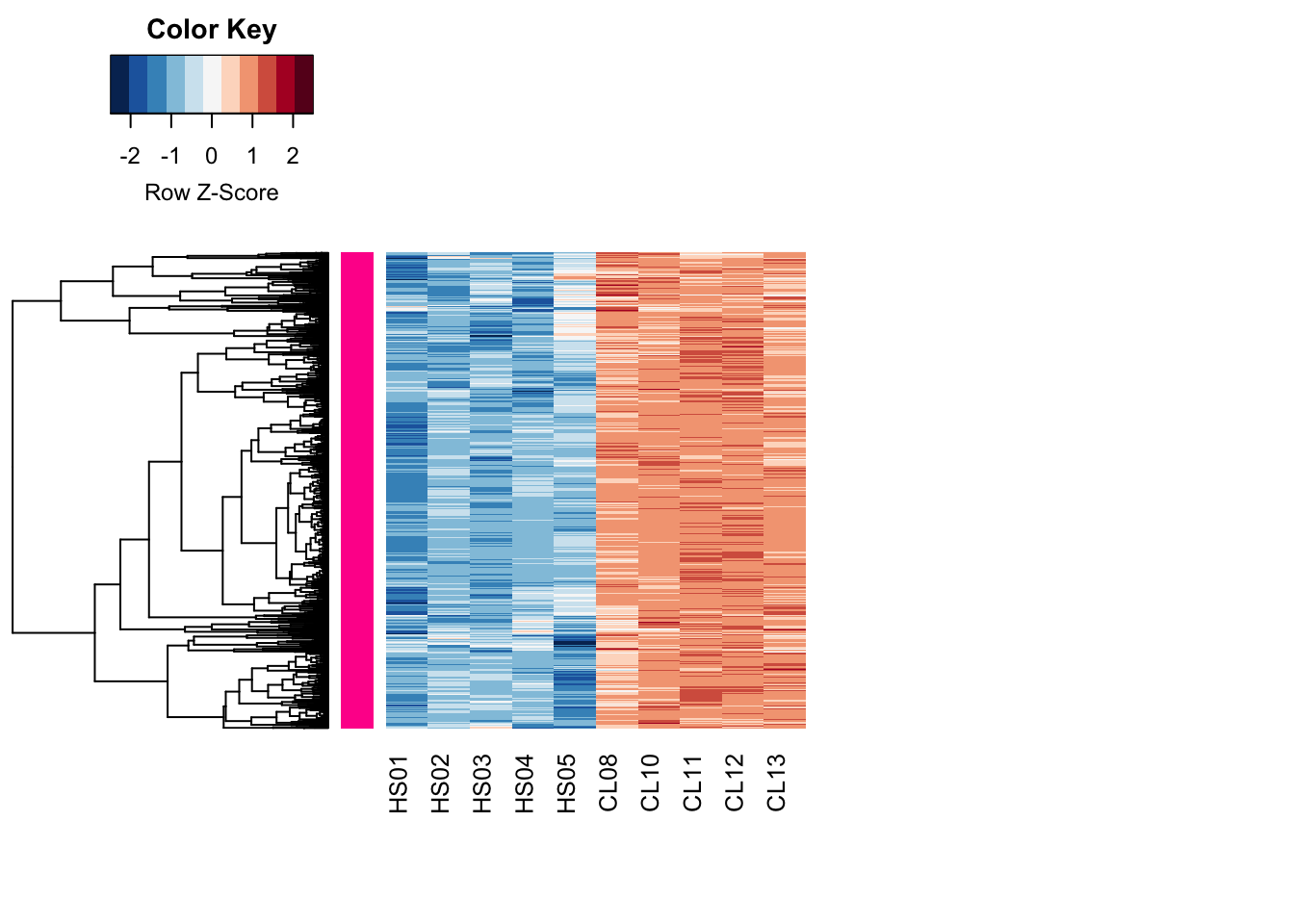
modulePick <- 2
Module_up <- diffGenes[names(module_assign[module_assign %in% modulePick]),]
hrsub_up <- hclust(
    as.dist(1 - cor(t(Module_up), method = "pearson")),
    method = "complete"
)

heatmap.2(
    Module_up,
    Rowv=as.dendrogram(hrsub_up),
    Colv=NA,
    labRow = NA,
    col=heatcolors, scale="row",
    density.info="none", trace="none",
    RowSideColors=module_color[module_assign%in%modulePick], margins=c(8,20)
)
modulePick <- 1
Module_down <- diffGenes[names(module_assign[module_assign %in% modulePick]),]
hrsub_down <- hclust(
    as.dist(1 - cor(t(Module_down), method = "pearson")),
    method = "complete"
)

heatmap.2(Module_down,
          Rowv=as.dendrogram(hrsub_down),
          Colv=NA,
          labRow = NA,
          col=heatcolors, scale="row",
          density.info="none", trace="none",
          RowSideColors=module_color[module_assign%in%modulePick], margins=c(8,20))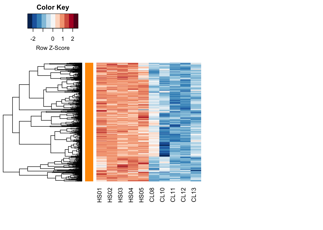
Step8: Functional enrichment analysis
Go enrichment analysis
### carry out GO enrichment using gProfiler2
#### use topTable result to pick the top genes for carrying out a Gene Ontology (GO) enrichment analysis
myTopHits <- topTable(
    ebFit,
    adjust = "BH",
    coef = 1,
    number = 50,
    sort.by = "logFC"
)

### use the 'gost' function from the gprofiler2 package to run GO enrichment analysis
gost_res <- gost(
    rownames(myTopHits),
    organism = "hsapiens",
    correction_method = "fdr"
)

### produce an interactive manhattan plot of enriched GO terms
gostplot(gost_res, interactive = TRUE, capped = T)
### produce a publication quality static manhattan plot with specific GO terms highlighted
mygostplot <- gostplot(
  gost_res,
  interactive = FALSE,
  capped = TRUE #set interactive=FALSE to get plot for publications
)

### rerun the above gostplot function with 'interactive=F' and save to an object 'mygostplot'
publish_gostplot(
  mygostplot, #your static gostplot from above
  highlight_terms = c("GO:0034987"),
  filename = NULL,
  width = NA,
  height = NA)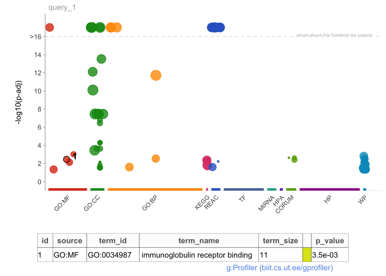

### generate a table of  gost results
publish_gosttable(
  gost_res,
  highlight_terms = NULL,
  use_colors = TRUE,
  show_columns = c("source", "term_name", "term_size", "intersection_size"),
  filename = NULL,
  ggplot=TRUE)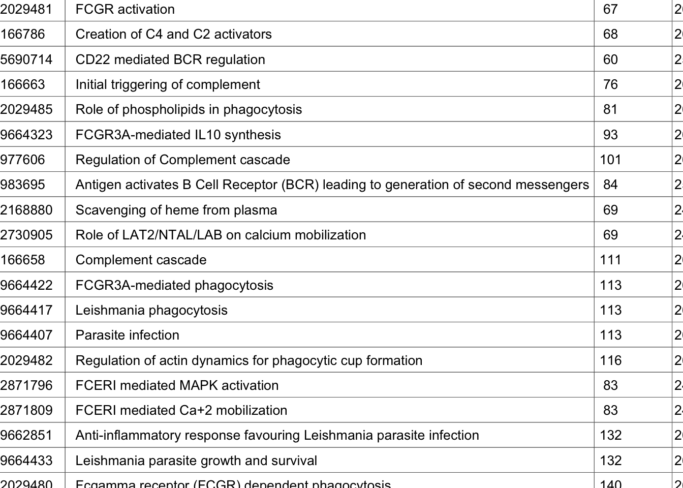
# now repeat the above steps using only genes from a single module from the step 6 script, by using `rownames(myModule)`
# what is value in breaking up DEGs into modules for functional enrichment analysis?
Perform GSEA using clusterProfiler
There are a few ways to get msigDB collections into R:
- Option1: download directly from msigdb and load from your computer. can use the ‘read.gmt’ function from clusterProfiler package to create a dataframe. alternatively, you can read in using ‘getGmt’ function from GSEABase package if you need a GeneSetCollection object
c2cp <- read.gmt("/Users/.../MSigDB/c2.cp.v7.1.symbols.gmt")- Option2: use the msigdb package to access up-to-date collections. this option has the additional advantage of providing access to species-specific collections are also retrieved as tibbles
msigdbr_species()
## # A tibble: 20 × 2
## species_name species_common_name
## <chr> <chr>
## 1 Anolis carolinensis Carolina anole, green anole
## 2 Bos taurus bovine, cattle, cow, dairy cow, domestic cat…
## 3 Caenorhabditis elegans <NA>
## 4 Canis lupus familiaris dog, dogs
## 5 Danio rerio leopard danio, zebra danio, zebra fish, zebr…
## 6 Drosophila melanogaster fruit fly
## 7 Equus caballus domestic horse, equine, horse
## 8 Felis catus cat, cats, domestic cat
## 9 Gallus gallus bantam, chicken, chickens, Gallus domesticus
## 10 Homo sapiens human
## 11 Macaca mulatta rhesus macaque, rhesus macaques, Rhesus monk…
## 12 Monodelphis domestica gray short-tailed opossum
## 13 Mus musculus house mouse, mouse
## 14 Ornithorhynchus anatinus duck-billed platypus, duckbill platypus, pla…
## 15 Pan troglodytes chimpanzee
## 16 Rattus norvegicus brown rat, Norway rat, rat, rats
## 17 Saccharomyces cerevisiae baker's yeast, brewer's yeast, S. cerevisiae
## 18 Schizosaccharomyces pombe 972h- <NA>
## 19 Sus scrofa pig, pigs, swine, wild boar
## 20 Xenopus tropicalis tropical clawed frog, western clawed frog
### Gets all collections/signatures with human gene IDs
hs_gsea <- msigdbr(species = "Homo sapiens")
### Take a look at the categories and subcategories of signatures available to you
hs_gsea |>
distinct(gs_cat, gs_subcat) |>
arrange(gs_cat, gs_subcat)
## # A tibble: 23 × 2
## gs_cat gs_subcat
## <chr> <chr>
## 1 C1 ""
## 2 C2 "CGP"
## 3 C2 "CP"
## 4 C2 "CP:BIOCARTA"
## 5 C2 "CP:KEGG"
## 6 C2 "CP:PID"
## 7 C2 "CP:REACTOME"
## 8 C2 "CP:WIKIPATHWAYS"
## 9 C3 "MIR:MIRDB"
## 10 C3 "MIR:MIR_Legacy"
## # ℹ 13 more rows
### Choose a specific msigdb collection/subcollection
hs_gsea_c2 <- msigdbr(
### change depending on species your data came from
species = "Homo sapiens",
category = "C2"
) |>
###just get the columns corresponding to signature name and gene symbols of genes in each signature
select(gs_name, gene_symbol)
### Pull out just the columns corresponding to gene symbols and LogFC for at least one pairwise comparison for the enrichment analysis
mydata_df_sub <- select(mydata_df, geneID, LogFC)
### Construct a named vector
mydata_gsea <- mydata_df_sub$LogFC
names(mydata_gsea) <- as.character(mydata_df_sub$geneID)
mydata_gsea <- sort(mydata_gsea, decreasing = TRUE)
### Run GSEA using the 'GSEA' function from clusterProfiler
myGSEA_res <- GSEA(mydata_gsea, TERM2GENE=hs_gsea_c2, verbose=FALSE)
myGSEA_df <- as_tibble(myGSEA_res@result)
### View results as an interactive table
# datatable(
# myGSEA_df,
# extensions = c('KeyTable', "FixedHeader"),
# caption = 'Signatures enriched in leishmaniasis',
# options = list(
# keys = TRUE,
# searchHighlight = TRUE,
# pageLength = 10,
# lengthMenu = c("10", "25", "50", "100")
# )
# ) |>
# formatRound(columns = c(2:10), digits = 2)
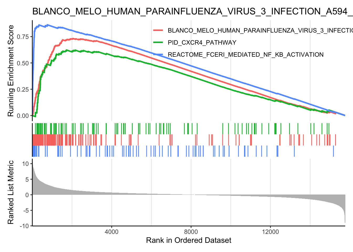
### Create enrichment plots using the enrichplot package
gseaplot2(
myGSEA_res,
### can choose multiple signatures to overlay in this plot
geneSetID = c(6, 47, 262),
### can set this to FALSE for a cleaner plot
pvalue_table = FALSE,
### can also turn off this title
title = myGSEA_res$Description[47]
) 
### Add a variable to this result that matches enrichment direction with phenotype
myGSEA_df <- myGSEA_df |>
    mutate(
        phenotype = case_when(
            NES > 0 ~ "disease",
            NES < 0 ~ "healthy"
        )
    )

### Create 'bubble plot' to summarize y signatures across x phenotypes
ggplot(myGSEA_df[1:20,], aes(x=phenotype, y=ID)) +
  geom_point(aes(size=setSize, color = NES, alpha=-log10(p.adjust))) +
  scale_color_gradient(low="blue", high="red") +
  theme_bw()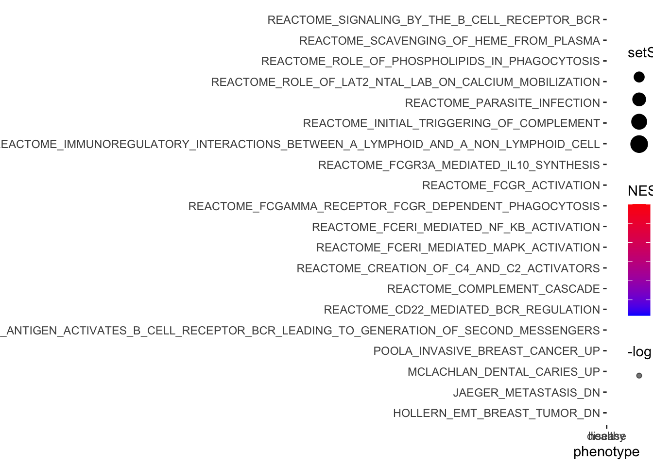
Competitive GSEA using CAMERA
For competitive tests the null hypothesis is that genes in the set are, at most, as often differentially expressed as genes outside the set.
### Create a few signatures to test in our enrichment analysis
### if your own data is from mice, wrap this in 'toupper()' to make gene symbols all caps
mySig <- rownames(myTopHits)

mySig2 <- sample(
  (rownames(v_DEGList_filtered_norm$E)),
  size = 50, replace = FALSE
  )

collection <- list(real = mySig, fake = mySig2)

###Test for enrichment using CAMERA
camera_res <- camera(v_DEGList_filtered_norm$E, collection, design, contrast_matrix[,1])
camera_df <- as_tibble(camera_res, rownames = "setName")
camera_df
## # A tibble: 2 × 5
##   setName NGenes Direction   PValue      FDR
##   <chr>    <dbl> <chr>        <dbl>    <dbl>
## 1 real        50 Up        5.85e-20 1.17e-19
## 2 fake        50 Up        9.57e- 1 9.57e- 1
Self-contained GSEA using ROAST
For self-contained the null hypothesis is that no genes in the set are differentially expressed.
mroast(
  v_DEGList_filtered_norm$E,
  collection, design,
  #mroast adjusts for multiple testing
  contrast=1
  )
##      NGenes PropDown PropUp Direction PValue   FDR PValue.Mixed FDR.Mixed
## real     50     0.06   0.94        Up  5e-04 5e-04        5e-04     5e-04
## fake     50     0.04   0.86        Up  5e-04 5e-04        5e-04     5e-04

### Repeat with an actual gene set collection
### camera requires collections to be presented as a list, rather than a tibble, so we must read in our signatures using the 'getGmt' function
broadSet_C2_ALL <- getGmt(
    here("learn", "DIY_Transcriptomics", "data", "c2.all.v7.2.symbols.gmt"),
    geneIdType = SymbolIdentifier()
)

### Extract as a list
broadSet_C2_ALL <- geneIds(broadSet_C2_ALL)
camera_res <- camera(
    v_DEGList_filtered_norm$E,
    broadSet_C2_ALL, design,
    contrast_matrix[, 1]
)
camera_df <- as_tibble(camera_res, rownames = "setName")
camera_df
## # A tibble: 6,229 × 5
##    setName                                    NGenes Direction   PValue      FDR
##    <chr>                                       <dbl> <chr>        <dbl>    <dbl>
##  1 MCLACHLAN_DENTAL_CARIES_UP                    245 Up        2.80e-33 1.74e-29
##  2 POOLA_INVASIVE_BREAST_CANCER_UP               275 Up        2.59e-32 8.06e-29
##  3 WIELAND_UP_BY_HBV_INFECTION                    99 Up        2.10e-31 4.36e-28
##  4 REACTOME_IMMUNOREGULATORY_INTERACTIONS_BE…    158 Up        9.85e-31 1.53e-27
##  5 REACTOME_FCGR_ACTIVATION                       62 Up        1.88e-29 2.34e-26
##  6 REACTOME_CD22_MEDIATED_BCR_REGULATION          53 Up        2.62e-27 2.72e-24
##  7 REACTOME_CREATION_OF_C4_AND_C2_ACTIVATORS      58 Up        1.70e-26 1.52e-23
##  8 REACTOME_INITIAL_TRIGGERING_OF_COMPLEMENT      66 Up        2.81e-26 2.19e-23
##  9 WALLACE_PROSTATE_CANCER_RACE_UP               277 Up        6.49e-26 4.49e-23
## 10 FLECHNER_BIOPSY_KIDNEY_TRANSPLANT_REJECTE…     86 Up        4.32e-25 2.69e-22
## # ℹ 6,219 more rows

### Filter based on FDR and display as interactive table
camera_df <- filter(camera_df, FDR<=0.01)

# datatable(
#     camera_df,
#     extensions = c('KeyTable', "FixedHeader"),
#     caption = 'Signatures enriched in leishmaniasis',
#     options = list(
#         keys = TRUE,
#         searchHighlight = TRUE,
#         pageLength = 10,
#         lengthMenu = c("10", "25", "50", "100")
#     )
# ) |>
#     formatRound(columns = c(2, 4, 5), digits = 2)

### Add a variable that maps up/down regulated pathways with phenotype
camera_df <- camera_df |>
    mutate(
        phenotype = case_when(
            Direction == "Up" ~ "disease",
            Direction == "Down" ~ "healthy"
        )
    )

### Filtering to return anything that has 'CD8' or 'CYTOTOX' in the name of the signature
camera_df_sub <- camera_df |>
  filter(str_detect(setName, "CD8|CYTOTOX"))

### Graph camera results as bubble chart
ggplot(camera_df[1:25,], aes(x=phenotype, y=setName)) +
  geom_point(aes(size=NGenes, color = Direction, alpha=-log10(FDR))) +
  theme_bw()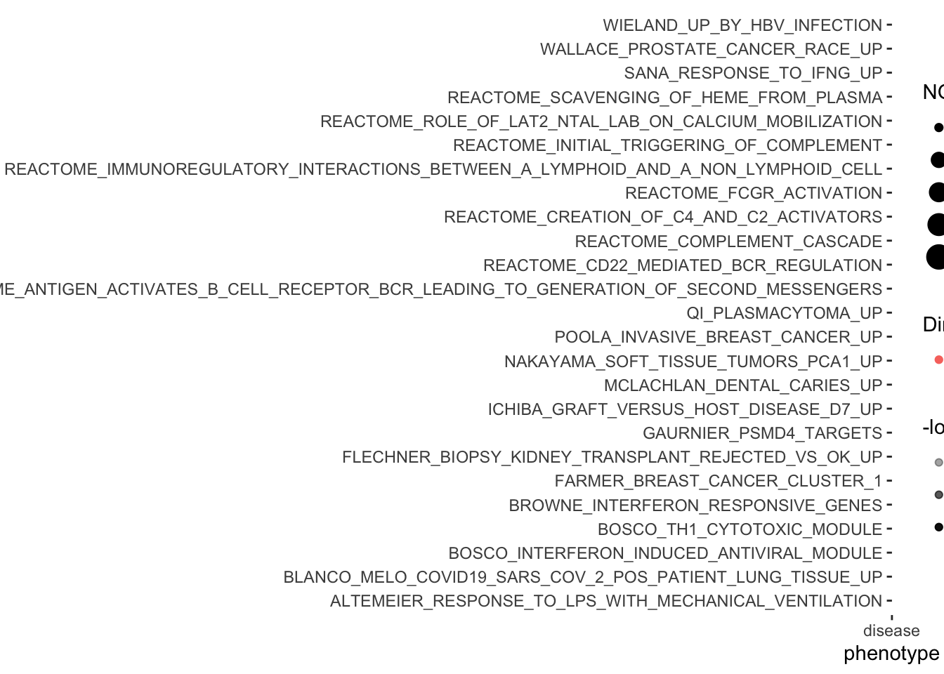
Single sample GSEA using the GSVA package
The GSVA package offers a different way of approaching functional enrichment analysis.
- In contrast to most GSE methods, GSVA performs a change in coordinate systems,transforming the data from a gene by sample matrix to a gene set (signature) by sample matrix. This allows for the evaluation of pathway enrichment for each sample.
- The method is both non-parametric and unsupervised bypasses the conventional approach of explicitly modeling phenotypes within enrichment scoring algorithms.
- Focus is therefore placed on the RELATIVE enrichment of pathways across the sample space rather than the absolute enrichment with respect to a phenotype. However, with data with a moderate to small sample size (< 30), other GSE methods that explicitly include the phenotype in their model are more likely to provide greater statistical power to detect functional enrichment.
# Be aware that if you choose a large MsigDB file here, this step may take a while
GSVA_res_C2CP <- gsva(
v_DEGList_filtered_norm$E,
### signatures
broadSet_C2_ALL,
### criteria for filtering gene sets
min.sz = 5, max.sz = 500,
mx.diff = FALSE,
### options for method are "gsva", ssgsea', "zscore" or "plage"
method = "gsva"
)
## Estimating GSVA scores for 5919 gene sets.
## Estimating ECDFs with Gaussian kernels
##
|
| | 0%
|
| | 1%
|
|= | 1%
|
|= | 2%
|
|== | 2%
|
|== | 3%
|
|== | 4%
|
|=== | 4%
|
|=== | 5%
|
|==== | 5%
|
|==== | 6%
|
|===== | 6%
|
|===== | 7%
|
|===== | 8%
|
|====== | 8%
|
|====== | 9%
|
|======= | 9%
|
|======= | 10%
|
|======= | 11%
|
|======== | 11%
|
|======== | 12%
|
|========= | 12%
|
|========= | 13%
|
|========= | 14%
|
|========== | 14%
|
|========== | 15%
|
|=========== | 15%
|
|=========== | 16%
|
|============ | 16%
|
|============ | 17%
|
|============ | 18%
|
|============= | 18%
|
|============= | 19%
|
|============== | 19%
|
|============== | 20%
|
|============== | 21%
|
|=============== | 21%
|
|=============== | 22%
|
|================ | 22%
|
|================ | 23%
|
|================ | 24%
|
|================= | 24%
|
|================= | 25%
|
|================== | 25%
|
|================== | 26%
|
|=================== | 26%
|
|=================== | 27%
|
|=================== | 28%
|
|==================== | 28%
|
|==================== | 29%
|
|===================== | 29%
|
|===================== | 30%
|
|===================== | 31%
|
|====================== | 31%
|
|====================== | 32%
|
|======================= | 32%
|
|======================= | 33%
|
|======================= | 34%
|
|======================== | 34%
|
|======================== | 35%
|
|========================= | 35%
|
|========================= | 36%
|
|========================== | 36%
|
|========================== | 37%
|
|========================== | 38%
|
|=========================== | 38%
|
|=========================== | 39%
|
|============================ | 39%
|
|============================ | 40%
|
|============================ | 41%
|
|============================= | 41%
|
|============================= | 42%
|
|============================== | 42%
|
|============================== | 43%
|
|============================== | 44%
|
|=============================== | 44%
|
|=============================== | 45%
|
|================================ | 45%
|
|================================ | 46%
|
|================================= | 46%
|
|================================= | 47%
|
|================================= | 48%
|
|================================== | 48%
|
|================================== | 49%
|
|=================================== | 49%
|
|=================================== | 50%
|
|=================================== | 51%
|
|==================================== | 51%
|
|==================================== | 52%
|
|===================================== | 52%
|
|===================================== | 53%
|
|===================================== | 54%
|
|====================================== | 54%
|
|====================================== | 55%
|
|======================================= | 55%
|
|======================================= | 56%
|
|======================================== | 56%
|
|======================================== | 57%
|
|======================================== | 58%
|
|========================================= | 58%
|
|========================================= | 59%
|
|========================================== | 59%
|
|========================================== | 60%
|
|========================================== | 61%
|
|=========================================== | 61%
|
|=========================================== | 62%
|
|============================================ | 62%
|
|============================================ | 63%
|
|============================================ | 64%
|
|============================================= | 64%
|
|============================================= | 65%
|
|============================================== | 65%
|
|============================================== | 66%
|
|=============================================== | 66%
|
|=============================================== | 67%
|
|=============================================== | 68%
|
|================================================ | 68%
|
|================================================ | 69%
|
|================================================= | 69%
|
|================================================= | 70%
|
|================================================= | 71%
|
|================================================== | 71%
|
|================================================== | 72%
|
|=================================================== | 72%
|
|=================================================== | 73%
|
|=================================================== | 74%
|
|==================================================== | 74%
|
|==================================================== | 75%
|
|===================================================== | 75%
|
|===================================================== | 76%
|
|====================================================== | 76%
|
|====================================================== | 77%
|
|====================================================== | 78%
|
|======================================================= | 78%
|
|======================================================= | 79%
|
|======================================================== | 79%
|
|======================================================== | 80%
|
|======================================================== | 81%
|
|========================================================= | 81%
|
|========================================================= | 82%
|
|========================================================== | 82%
|
|========================================================== | 83%
|
|========================================================== | 84%
|
|=========================================================== | 84%
|
|=========================================================== | 85%
|
|============================================================ | 85%
|
|============================================================ | 86%
|
|============================================================= | 86%
|
|============================================================= | 87%
|
|============================================================= | 88%
|
|============================================================== | 88%
|
|============================================================== | 89%
|
|=============================================================== | 89%
|
|=============================================================== | 90%
|
|=============================================================== | 91%
|
|================================================================ | 91%
|
|================================================================ | 92%
|
|================================================================= | 92%
|
|================================================================= | 93%
|
|================================================================= | 94%
|
|================================================================== | 94%
|
|================================================================== | 95%
|
|=================================================================== | 95%
|
|=================================================================== | 96%
|
|==================================================================== | 96%
|
|==================================================================== | 97%
|
|==================================================================== | 98%
|
|===================================================================== | 98%
|
|===================================================================== | 99%
|
|======================================================================| 99%
|
|======================================================================| 100%- Apply linear model to GSVA result. Now using Limma to find significantly enriched gene sets in the same way you did to find diffGenes. This means you’ll be using topTable, decideTests, etc.
- note that you need to reference your design and contrast matrix here.
fit_C2CP <- lmFit(GSVA_res_C2CP, design)
ebfit_C2CP <- eBayes(fit_C2CP)
### Use topTable and decideTests functions to identify the differentially enriched gene sets
topPaths_C2CP <- topTable(ebfit_C2CP, adjust ="BH", coef=1, number=50, sort.by="logFC")
res_C2CP <- decideTests(ebfit_C2CP, method="global", adjust.method="BH", p.value=0.05, lfc=0.58)
### The summary of the decideTests result shows how many sets were enriched in induced and repressed genes in all sample types
summary(res_C2CP)
## disease healthy
## Down 12 42
## NotSig 5851 5864
## Up 56 13
# Pull out the gene sets that are differentially enriched between groups
diffSets_C2CP <- GSVA_res_C2CP[res_C2CP[,1] !=0,]
head(diffSets_C2CP)
## HS01 HS02 HS03
## ST_IL_13_PATHWAY -0.7173858 -0.7147717 -0.7164712
## WATANABE_ULCERATIVE_COLITIS_WITH_CANCER_DN -0.6188325 -0.5710992 -0.4131349
## FARMER_BREAST_CANCER_CLUSTER_1 -0.6886216 -0.5784651 -0.5593251
## BOWIE_RESPONSE_TO_EXTRACELLULAR_MATRIX -0.6707584 -0.5317945 -0.5360570
## BOWIE_RESPONSE_TO_TAMOXIFEN -0.6717424 -0.5377614 -0.5172726
## KAUFFMANN_MELANOMA_RELAPSE_DN 0.5698331 0.7398284 0.6624807
## HS04 HS05 CL08
## ST_IL_13_PATHWAY -0.5968289 -0.4130711 0.8128353
## WATANABE_ULCERATIVE_COLITIS_WITH_CANCER_DN -0.6270975 -0.5185058 0.2930852
## FARMER_BREAST_CANCER_CLUSTER_1 -0.6325020 -0.4714246 0.5083211
## BOWIE_RESPONSE_TO_EXTRACELLULAR_MATRIX -0.6457163 -0.5252770 0.5529664
## BOWIE_RESPONSE_TO_TAMOXIFEN -0.6692727 -0.5128578 0.5408430
## KAUFFMANN_MELANOMA_RELAPSE_DN 0.4426951 0.6730961 -0.6256108
## CL10 CL11 CL12
## ST_IL_13_PATHWAY 0.6256980 0.5670608 0.6341371
## WATANABE_ULCERATIVE_COLITIS_WITH_CANCER_DN 0.5838839 0.6787619 0.7118710
## FARMER_BREAST_CANCER_CLUSTER_1 0.5593513 0.6517882 0.7463300
## BOWIE_RESPONSE_TO_EXTRACELLULAR_MATRIX 0.4914990 0.7723819 0.6409015
## BOWIE_RESPONSE_TO_TAMOXIFEN 0.5064169 0.7568069 0.6405129
## KAUFFMANN_MELANOMA_RELAPSE_DN -0.6277048 -0.6895166 -0.8205882
## CL13
## ST_IL_13_PATHWAY 0.6455147
## WATANABE_ULCERATIVE_COLITIS_WITH_CANCER_DN 0.6389032
## FARMER_BREAST_CANCER_CLUSTER_1 0.5802493
## BOWIE_RESPONSE_TO_EXTRACELLULAR_MATRIX 0.6434423
## BOWIE_RESPONSE_TO_TAMOXIFEN 0.6232986
## KAUFFMANN_MELANOMA_RELAPSE_DN -0.3907835
dim(diffSets_C2CP)
## [1] 68 10
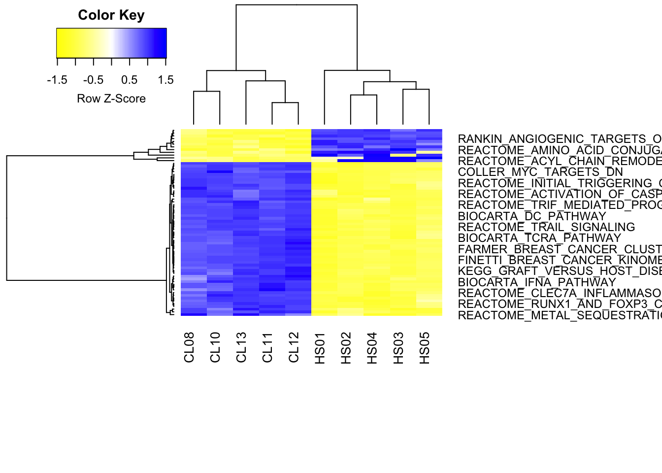
### Make a heatmap of differentially enriched gene sets
hr_C2CP <- hclust(
as.dist(1 - cor(t(diffSets_C2CP), method = "pearson")),
### cluster rows by pearson correlation
method = "complete"
)
hc_C2CP <- hclust(
as.dist(1 - cor(diffSets_C2CP, method = "spearman")),
### cluster columns by spearman correlation
method = "complete"
)
### Cut the resulting tree and create color vector for clusters. Vary the cut height to give more or fewer clusters, or you the 'k' argument to force n number of clusters
mycl_C2CP <- cutree(hr_C2CP, k=2)
mycolhc_C2CP <- rainbow(
length(unique(mycl_C2CP)),
start = 0.1, end = 0.9
)
mycolhc_C2CP <- mycolhc_C2CP[as.vector(mycl_C2CP)]
### assign your favorite heatmap color scheme. Some useful examples: colorpanel(40, "darkblue", "yellow", "white"); heat.colors(75); cm.colors(75); rainbow(75); redgreen(75); library(RColorBrewer); rev(brewer.pal(9,"Blues")[-1]). Type demo.col(20) to see more color schemes.
myheatcol <- colorRampPalette(colors=c("yellow","white","blue"))(100)
### Plot the hclust results as a heatmap
heatmap.2(
diffSets_C2CP,
Rowv = as.dendrogram(hr_C2CP),
Colv = as.dendrogram(hc_C2CP),
col = myheatcol, scale = "row",
density.info = "none", trace = "none",
### Creates heatmap for entire data set where the obtained clusters are indicated in the color bar.
cexRow = 0.9, cexCol = 1, margins = c(10, 14)
) 
Reference
SessionInfo
sessionInfo()
## R version 4.3.1 (2023-06-16)
## Platform: aarch64-apple-darwin20 (64-bit)
## Running under: macOS Sonoma 14.1.1
##
## Matrix products: default
## BLAS:   /Library/Frameworks/R.framework/Versions/4.3-arm64/Resources/lib/libRblas.0.dylib
## LAPACK: /Library/Frameworks/R.framework/Versions/4.3-arm64/Resources/lib/libRlapack.dylib;  LAPACK version 3.11.0
##
## locale:
## [1] en_US.UTF-8/en_US.UTF-8/en_US.UTF-8/C/en_US.UTF-8/en_US.UTF-8
##
## time zone: Asia/Singapore
## tzcode source: internal
##
## attached base packages:
## [1] stats4    stats     graphics  grDevices utils     datasets  methods
## [8] base
##
## other attached packages:
##  [1] enrichplot_1.20.0         msigdbr_7.5.1
##  [3] clusterProfiler_4.8.2     gprofiler2_0.2.2
##  [5] GSVA_1.48.3               GSEABase_1.62.0
##  [7] graph_1.78.0              annotate_1.80.0
##  [9] XML_3.99-0.15             gplots_3.1.3
## [11] heatmaply_1.5.0           viridis_0.6.4
## [13] viridisLite_0.4.2         RColorBrewer_1.1-3
## [15] gt_0.10.0                 plotly_4.10.3
## [17] DT_0.30                   cowplot_1.1.1
## [19] matrixStats_1.1.0         edgeR_4.0.1
## [21] limma_3.58.1              datapasta_3.1.0
## [23] here_1.0.1                EnsDb.Hsapiens.v86_2.99.0
## [25] ensembldb_2.24.1          AnnotationFilter_1.24.0
## [27] GenomicFeatures_1.52.2    AnnotationDbi_1.64.1
## [29] Biobase_2.62.0            GenomicRanges_1.52.1
## [31] GenomeInfoDb_1.38.0       IRanges_2.36.0
## [33] S4Vectors_0.40.1          BiocGenerics_0.48.1
## [35] tximport_1.28.0           lubridate_1.9.3
## [37] forcats_1.0.0             stringr_1.5.1
## [39] dplyr_1.1.4               purrr_1.0.2
## [41] readr_2.1.4               tidyr_1.3.0
## [43] tibble_3.2.1              ggplot2_3.4.4
## [45] tidyverse_2.0.0           rhdf5_2.44.0
##
## loaded via a namespace (and not attached):
##   [1] fs_1.6.3                    ProtGenerics_1.32.0
##   [3] bitops_1.0-7                HDO.db_0.99.1
##   [5] httr_1.4.7                  webshot_0.5.5
##   [7] tools_4.3.1                 utf8_1.2.4
##   [9] R6_2.5.1                    HDF5Array_1.28.1
##  [11] mgcv_1.9-0                  lazyeval_0.2.2
##  [13] rhdf5filters_1.12.1         withr_2.5.2
##  [15] prettyunits_1.2.0           gridExtra_2.3
##  [17] cli_3.6.1                   TSP_1.2-4
##  [19] scatterpie_0.2.1            sass_0.4.7
##  [21] labeling_0.4.3              commonmark_1.9.0
##  [23] Rsamtools_2.16.0            yulab.utils_0.1.0
##  [25] gson_0.1.0                  DOSE_3.26.2
##  [27] RSQLite_2.3.3               generics_0.1.3
##  [29] gridGraphics_0.5-1          BiocIO_1.10.0
##  [31] crosstalk_1.2.0             vroom_1.6.4
##  [33] gtools_3.9.5                dendextend_1.17.1
##  [35] GO.db_3.17.0                Matrix_1.6-3
##  [37] fansi_1.0.5                 abind_1.4-5
##  [39] lifecycle_1.0.4             yaml_2.3.7
##  [41] SummarizedExperiment_1.30.2 qvalue_2.32.0
##  [43] BiocFileCache_2.8.0         grid_4.3.1
##  [45] blob_1.2.4                  promises_1.2.1
##  [47] crayon_1.5.2                lattice_0.22-5
##  [49] beachmat_2.16.0             KEGGREST_1.42.0
##  [51] pillar_1.9.0                knitr_1.45
##  [53] fgsea_1.26.0                rjson_0.2.21
##  [55] codetools_0.2-19            fastmatch_1.1-4
##  [57] glue_1.6.2                  downloader_0.4
##  [59] ggfun_0.1.3                 data.table_1.14.8
##  [61] vctrs_0.6.4                 png_0.1-8
##  [63] treeio_1.24.3               gtable_0.3.4
##  [65] assertthat_0.2.1            cachem_1.0.8
##  [67] xfun_0.41                   mime_0.12
##  [69] S4Arrays_1.0.6              tidygraph_1.2.3
##  [71] SingleCellExperiment_1.22.0 seriation_1.4.2
##  [73] iterators_1.0.14            statmod_1.5.0
##  [75] ellipsis_0.3.2              nlme_3.1-163
##  [77] ggtree_3.8.2                bit64_4.0.5
##  [79] progress_1.2.2              filelock_1.0.2
##  [81] rprojroot_2.0.4             irlba_2.3.5.1
##  [83] KernSmooth_2.23-22          colorspace_2.1-0
##  [85] DBI_1.1.3                   tidyselect_1.2.0
##  [87] bit_4.0.5                   compiler_4.3.1
##  [89] curl_5.1.0                  xml2_1.3.5
##  [91] DelayedArray_0.26.7         shadowtext_0.1.2
##  [93] rtracklayer_1.60.1          scales_1.2.1
##  [95] caTools_1.18.2              hexbin_1.28.3
##  [97] rappdirs_0.3.3              digest_0.6.33
##  [99] rmarkdown_2.25              ca_0.71.1
## [101] XVector_0.42.0              htmltools_0.5.7
## [103] pkgconfig_2.0.3             sparseMatrixStats_1.12.2
## [105] MatrixGenerics_1.14.0       dbplyr_2.4.0
## [107] fastmap_1.1.1               rlang_1.1.2
## [109] htmlwidgets_1.6.2           shiny_1.8.0
## [111] DelayedMatrixStats_1.22.6   farver_2.1.1
## [113] jsonlite_1.8.7              BiocParallel_1.36.0
## [115] GOSemSim_2.26.1             BiocSingular_1.16.0
## [117] RCurl_1.98-1.13             magrittr_2.0.3
## [119] GenomeInfoDbData_1.2.11     ggplotify_0.1.2
## [121] patchwork_1.1.3             Rhdf5lib_1.22.1
## [123] munsell_0.5.0               Rcpp_1.0.11
## [125] ape_5.7-1                   babelgene_22.9
## [127] stringi_1.8.1               ggraph_2.1.0
## [129] zlibbioc_1.48.0             MASS_7.3-60
## [131] plyr_1.8.9                  parallel_4.3.1
## [133] ggrepel_0.9.4               Biostrings_2.70.1
## [135] graphlayouts_1.0.2          splines_4.3.1
## [137] hms_1.1.3                   locfit_1.5-9.8
## [139] igraph_1.5.1                markdown_1.11
## [141] reshape2_1.4.4              biomaRt_2.56.1
## [143] ScaledMatrix_1.8.1          evaluate_0.23
## [145] httpuv_1.6.12               tzdb_0.4.0
## [147] foreach_1.5.2               tweenr_2.0.2
## [149] polyclip_1.10-6             ggforce_0.4.1
## [151] rsvd_1.0.5                  xtable_1.8-4
## [153] restfulr_0.0.15             tidytree_0.4.5
## [155] later_1.3.1                 aplot_0.2.2
## [157] memoise_2.0.1               registry_0.5-1
## [159] GenomicAlignments_1.36.0    timechange_0.2.0