### Load packages
pacman::p_load(
    tidyverse,  # tidy data
    FactoMineR, # compute principal component methods
    factoextra,  # extract, visualize and interpretate the results
    corrplot,  # visualize cos2 of variables
    broom,
    ggforce,
    palmerpenguins,
    umap,
    Rtsne
)
Library and data
### load packages
rm(list = ls())
### demo data
penguins <- penguins |>
  drop_na() |>
  select(-year)
head(penguins)
## # A tibble: 6 × 7
##   species island    bill_length_mm bill_depth_mm flipper_length_mm body_mass_g
##   <fct>   <fct>              <dbl>         <dbl>             <int>       <int>
## 1 Adelie  Torgersen           39.1          18.7               181        3750
## 2 Adelie  Torgersen           39.5          17.4               186        3800
## 3 Adelie  Torgersen           40.3          18                 195        3250
## 4 Adelie  Torgersen           36.7          19.3               193        3450
## 5 Adelie  Torgersen           39.3          20.6               190        3650
## 6 Adelie  Torgersen           38.9          17.8               181        3625
## # ℹ 1 more variable: sex <fct>
PCA
### Perform PCA using prcomp()
pca_fit <- penguins |>
  select(where(is.numeric)) |>
  scale() |>
  prcomp()

### importance of components
pca_fit
## Standard deviations (1, .., p=4):
## [1] 1.6569115 0.8821095 0.6071594 0.3284579
##
## Rotation (n x k) = (4 x 4):
##                          PC1         PC2        PC3        PC4
## bill_length_mm     0.4537532 -0.60019490 -0.6424951  0.1451695
## bill_depth_mm     -0.3990472 -0.79616951  0.4258004 -0.1599044
## flipper_length_mm  0.5768250 -0.00578817  0.2360952 -0.7819837
## body_mass_g        0.5496747 -0.07646366  0.5917374  0.5846861
summary(pca_fit)
## Importance of components:
##                           PC1    PC2     PC3     PC4
## Standard deviation     1.6569 0.8821 0.60716 0.32846
## Proportion of Variance 0.6863 0.1945 0.09216 0.02697
## Cumulative Proportion  0.6863 0.8809 0.97303 1.00000

### visualize the PC1 and PC2
pca_fit |>
  augment(penguins) |>
  rename_at(
    vars(starts_with(".fitted")),
    list(~str_replace(., ".fitted", ""))
    ) |>
    ggplot(aes(x = PC1, y = PC2, color = species, shape = sex)) +
    geom_point()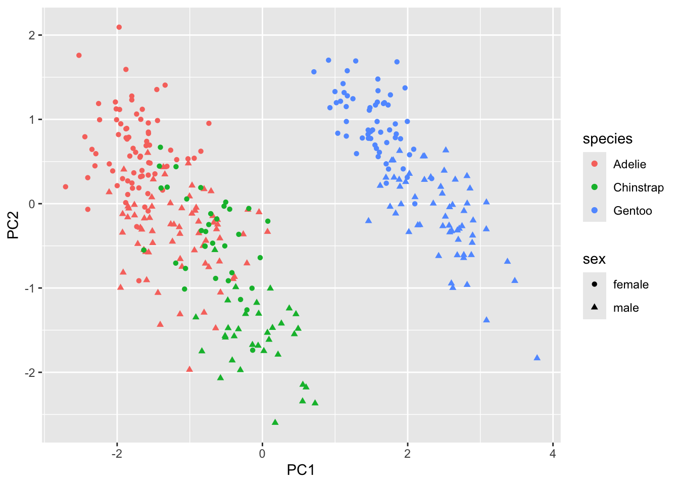
UMAP
rm(list = ls())
### theme set
theme_set(theme_bw(18))
### subset data
penguins <- penguins |>
  drop_na() |>
  select(-year) |>
  mutate(ID = row_number())

### meta data
penguins_meta <- penguins |>
  select(ID, species, island, sex)
### umap analysis
set.seed(123)
umap_fit <- penguins |>
  select(where(is.numeric)) |>
  column_to_rownames("ID") |>
  scale() |>
  umap()
### retrieve data from umap analysis
umap_df <- umap_fit$layout |>
  as.data.frame() |>
  rename(UMAP1 = "V1", UMAP2 = "V2") |>
  mutate(ID = row_number()) |>
  inner_join(penguins_meta, by = "ID") |>
  as_tibble()
head(umap_df)
## # A tibble: 6 × 6
##   UMAP1 UMAP2    ID species island    sex
##   <dbl> <dbl> <int> <fct>   <fct>     <fct>
## 1 -7.00 -1.14     1 Adelie  Torgersen male
## 2 -5.79 -1.28     2 Adelie  Torgersen female
## 3 -5.39 -1.87     3 Adelie  Torgersen female
## 4 -7.55 -2.53     4 Adelie  Torgersen female
## 5 -8.77 -2.36     5 Adelie  Torgersen male
## 6 -6.22 -1.30     6 Adelie  Torgersen female
### visualize umap
umap_df |>
  ggplot(aes(x = UMAP1, y = UMAP2, color = species, shape = sex)) +
  geom_point() +
  labs(x = "UMAP1", y = "UMAP2", title = "UMAP plot")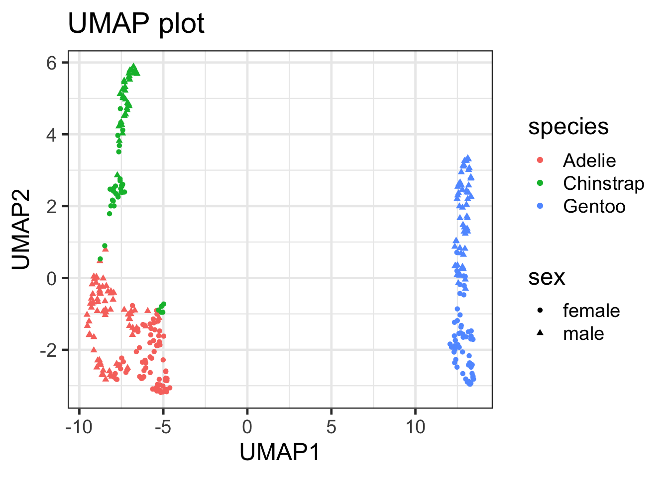
### facet by island
umap_df |>
  ggplot(aes(x = UMAP1, y = UMAP2, color = species))+
  geom_point(size = 3, alpha = 0.5) +
  facet_wrap(~island) +
  labs(x = "UMAP1", y = "UMAP2", subtitle = "UMAP plot") +
  theme(legend.position = "bottom")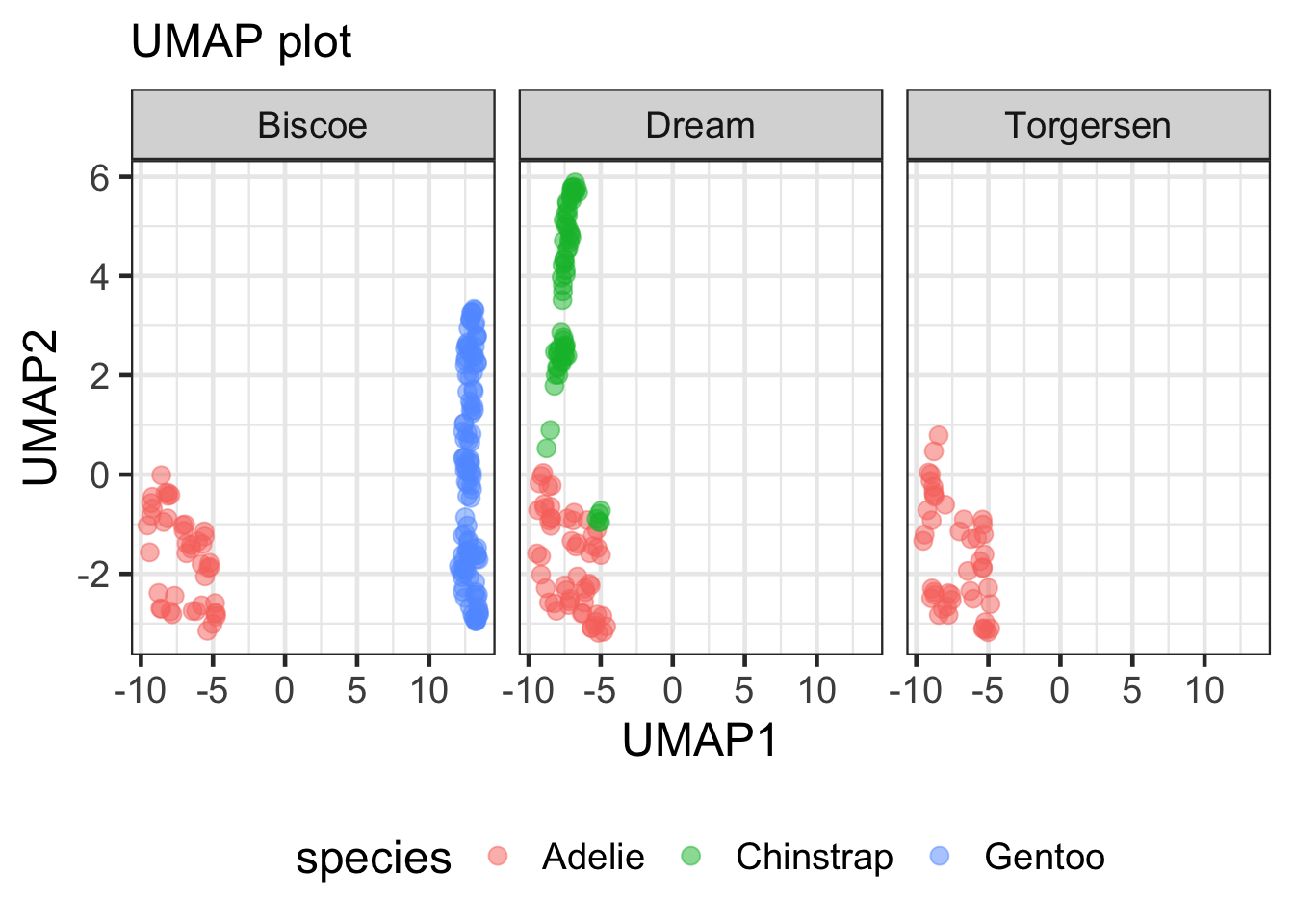
### circlize the outlier cases
umap_df |>
  ggplot(aes(x = UMAP1, y = UMAP2, color = species, shape = sex)) +
  geom_point()+
  labs(x = "UMAP1", y = "UMAP2", subtitle = "UMAP plot") +
  geom_circle(aes(x0 = -5, y0= -3.8, r = 0.65), color = "green", inherit.aes = FALSE)
## Warning in geom_circle(aes(x0 = -5, y0 = -3.8, r = 0.65), color = "green", : All aesthetics have length 1, but the data has 333 rows.
## ℹ Did you mean to use `annotate()`?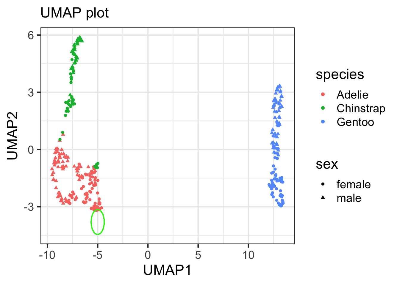
tSNE
rm(list = ls())
### theme set
theme_set(theme_bw(18))
### subset data
penguins <- penguins |>
drop_na() |>
select(-year) |>
mutate(ID = row_number())
### meta data
penguins_meta <- penguins |>
select(ID, species, island, sex)
### tSNE analysis
set.seed(135)
tsne_fit <- penguins |>
select(where(is.numeric)) |>
column_to_rownames("ID") |>
scale() |>
Rtsne()
### retrive data
tsne_df <- tsne_fit$Y |>
as.data.frame() |>
rename(tSNE1 = "V1", tSNE2 = "V2") |>
mutate(ID = row_number())
tsne_df <- tsne_df |>
inner_join(penguins_meta, by = "ID")
### check data
head(tsne_df)
## tSNE1 tSNE2 ID species island sex
## 1 -5.788624 5.231530 1 Adelie Torgersen male
## 2 -6.308533 8.950800 2 Adelie Torgersen female
## 3 -6.015678 12.082790 3 Adelie Torgersen female
## 4 -9.649822 6.857170 4 Adelie Torgersen female
## 5 -12.064101 4.828783 5 Adelie Torgersen male
## 6 -5.480114 7.486022 6 Adelie Torgersen female
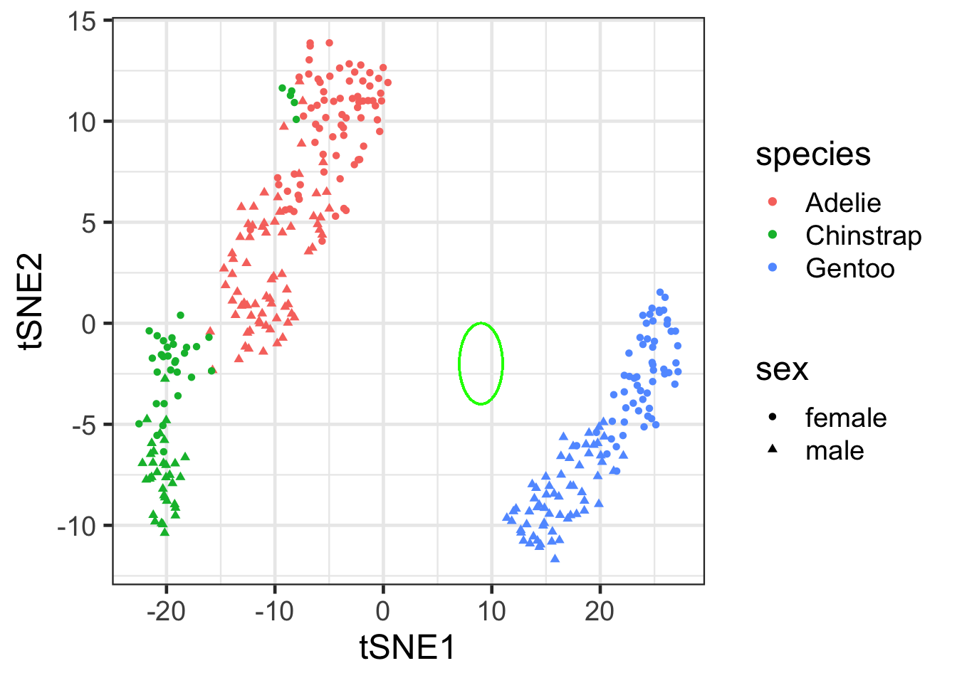
### visualize
tsne_df |>
ggplot(
aes(x = tSNE1, y = tSNE2, color = species, shape = sex)) +
geom_point()+
theme(legend.position = "right") +
### identify potential sample mismatch
geom_circle(
aes(x0 = 9, y0 = -2, r = 2),
color = "green",
inherit.aes = FALSE
)
## Warning in geom_circle(aes(x0 = 9, y0 = -2, r = 2), color = "green", inherit.aes = FALSE): All aesthetics have length 1, but the data has 333 rows.
## ℹ Did you mean to use `annotate()`?